pbc <- survival::pbc %>%
  as_tibble() %>%
  clean_names() %>%
  mutate(
    died      = as.integer(status == 2),
    trt       = factor(trt, levels = c(1, 2), labels = c("D-penicillamine", "Placebo")),
    sex       = factor(sex, levels = c("f", "m"), labels = c("Female", "Male")),
    stage     = factor(stage, levels = 1:4, labels = paste("Stage", 1:4)),
    log_bili  = log(bili),
    log_proto = log(protime)
  ) %>%
filter(!is.na(trt))17 Survival Analysis and Time-to-Event Data
ImportantBefore You Start
This session assumes you are comfortable with basic inference (hypothesis testing, p-values) and regression concepts. Complete at least the Hypothesis Testing and Linear Regression sessions before starting here.
NoteSession at a Glance
Total core time: ~180 minutes (about 3 hours). A natural break point is after Example 1 (the PBC survival curves and Cox models)—cover Example 2 and the exercises in a second sitting. Exercise 3 is open-ended and its time will vary.
| Section | Time | Type |
|---|---|---|
| The Key Idea: “Survived At Least…” | ~10 min | Concept |
| Background: Key Concepts | ~15 min | Concept |
| Example 1: Clinical Data (PBC) | ~60 min | Walkthrough |
| Example 2: Melanoma Data | ~20 min | Walkthrough |
| What Can Go Wrong | ~10 min | Reading |
| Exercise 1 (Guided) | ~15 min | Practice |
| Exercise 2 (Semi-guided) | ~20 min | Practice |
| Exercise 3 (Open-ended) | 15–30 min | Practice |
| Comprehension Check | ~10 min | Self-test |
If you are short on time, focus on the multivariable Cox model (cox_full) and its proportional-hazards check in Example 1 – together they show both how to adjust for multiple predictors and how to detect when the model’s central assumption does not hold.
TipHow to Use the Code in This Session
Every code chunk below is written so you can copy it into your R console (or an R script) and run it yourself, in the order shown. Where you see a “Run It Yourself” box, stop and run the code above it before reading the explanation that follows.
17.1 When Do You Use This?
Tip
Your outcome is the time until an event: death, disease recurrence, treatment response, or any clearly defined endpoint, and some participants did not experience the event by the end of observation (censored). Standard methods cannot handle censoring correctly because a censored observation is not a missing value: you know the person survived at least to that time. Survival analysis models both event probability and time to event while making full use of censored information.
NoteTeacher Note
Before starting, ask learners for their own “survived at least…” example: a patient who hasn’t relapsed yet, a machine part that hasn’t failed yet, a customer who hasn’t churned yet. Then ask: in the PBC liver disease data below, out of 312 patients with treatment information, roughly how many do you expect to have died by the end of follow-up – a quarter, a third, half? (The real answer, revealed in the log-rank test output, is 125 of 312, about 40%.) Holding a guess in mind makes the first KM plot land harder.
17.2 Learning Objectives
After completing this session you will be able to:
- Explain censoring and why ordinary regression cannot handle it
- Estimate and plot Kaplan-Meier survival curves and compare groups with the log-rank test
- Fit a Cox proportional hazards model and interpret hazard ratios
- Check the proportional hazards assumption using Schoenfeld residuals
- Extend the model to stratified and time-varying coefficient analyses
17.3 The Key Idea: What to Do with “Survived At Least…”
Estimated time: ~10 minutes (Concept)
Here is the problem that makes survival analysis different from everything else in this course.
You follow 100 patients for five years. At the end, 60 have died. The other 40 are alive, or were lost to follow-up, or withdrew. Can you use logistic regression on the “died/alive” outcome? No, because a patient who dropped out at year 1 is counted the same as one who stayed healthy for 4.9 years. You are throwing away timing information.
Can you use linear regression on time-to-death? No, because 40 patients have no death time. You can’t include them.
Survival analysis keeps everyone in the analysis: the 60 who died contribute their full event time, and the 40 who were censored contribute their partial time (they were at risk until they left). No one is wasted.
17.4 Background: Key Concepts
Estimated time: ~15 minutes (Concept)
17.4.1 Time-to-event data
Each patient contributes: - Event time \(T_i\): the time from study entry to the event (death, relapse, etc.) - Event indicator \(\delta_i\): 1 if the event occurred, 0 if censored
Right censoring is the most common type: the event has not happened by the time observation ends.
17.4.2 The Survival and Hazard Functions
The survival function \(S(t)\) is the probability of surviving past time \(t\):
\[S(t) = P(T > t)\]
The hazard function \(h(t)\) is the instantaneous rate of the event at time \(t\), given survival to \(t\):
\[h(t) = \lim_{\Delta t \to 0} \frac{P(t \leq T < t + \Delta t \mid T \geq t)}{\Delta t}\]
17.4.3 The Cox Proportional Hazards Model
The Cox model relates covariates to the hazard:
\[h(t \mid X) = h_0(t) \cdot \exp(\beta_1 X_1 + \cdots + \beta_p X_p)\]
The hazard ratio (HR) for a one-unit increase in \(X_j\) is \(e^{\beta_j}\). HR > 1 means increased risk; HR < 1 means reduced risk. The baseline hazard \(h_0(t)\) is left unspecified: this is the “semi-parametric” nature of the Cox model.
Proportional hazards assumption: The ratio of hazards between any two covariate patterns is constant over time. This must be checked.
17.5 Example 1: Clinical Data (PBC)
Estimated time: ~60 minutes (Walkthrough)
NoteTeacher Note
This example has several natural stopping points – pause and ask learners to predict before running each one:
- After
pbc-setup: thefilter(!is.na(trt))step quietly drops 106 of the 418 PBC patients (these are an observational follow-up cohort with no treatment assignment), leaving 312 for the trial comparison. Ask: does this filter introduce bias? (Worth discussing, but in this case the 106 are simply a separate cohort, not a non-random subset of the 312.) - Before
km-plot: D-penicillamine was the experimental drug in the real PBC trial. Ask learners to predict whether the two KM curves will separate. (They will not – the trial famously found no survival benefit.) - Before
cox-multi: ask which single predictor learners expect to have the strongest hazard ratio once everything is adjusted – bilirubin, albumin, or disease stage? (Bilirubin and albumin remain strong; stage becomes less precise once bilirubin and albumin are in the model, because they partly capture the same underlying liver damage.) - Before
ph-test: ask whether learners expect the proportional hazards assumption to hold perfectly for a 5-predictor model followed for over 10 years. (It does not – two terms show evidence of violation, a realistic outcome worth normalising.)
17.5.1 Prepare the Data
TipRun It Yourself
This chunk produces no printed output, but it does important work. Run nrow(pbc) afterwards: you should get 312, not 418. The filter(!is.na(trt)) step removes 106 patients who were enrolled in an observational follow-up registry without a randomised treatment assignment. Every analysis below (KM curves, log-rank test, Cox models) uses this 312-patient trial subset.
17.5.2 Kaplan-Meier Survival Curves
Estimated time: ~10 minutes (Walkthrough)
km_trt <- survfit(Surv(time, died) ~ trt, data = pbc)
summary(km_trt, times = c(365, 730, 1460, 2920))
Call: survfit(formula = Surv(time, died) ~ trt, data = pbc)
trt=D-penicillamine
time n.risk n.event survival std.err lower 95% CI upper 95% CI
365 149 9 0.943 0.0184 0.908 0.980
730 143 5 0.911 0.0226 0.868 0.957
1460 101 22 0.764 0.0346 0.699 0.834
2920 34 22 0.542 0.0482 0.455 0.645
trt=Placebo
time n.risk n.event survival std.err lower 95% CI upper 95% CI
365 141 13 0.916 0.0224 0.873 0.961
730 135 6 0.877 0.0265 0.826 0.930
1460 93 20 0.740 0.0360 0.672 0.814
2920 33 11 0.605 0.0486 0.517 0.709
TipRun It Yourself
You should see survival estimates at four follow-up times (1, 2, 4, and 8 years):
| Time (days) | D-penicillamine | Placebo |
|---|---|---|
| 365 | 0.943 (0.908–0.980) | 0.916 (0.873–0.961) |
| 730 | 0.911 (0.868–0.957) | 0.877 (0.826–0.930) |
| 1460 | 0.764 (0.699–0.834) | 0.740 (0.672–0.814) |
| 2920 | 0.542 (0.455–0.645) | 0.605 (0.517–0.709) |
At every time point the two groups’ confidence intervals overlap substantially – a first hint that treatment makes little difference, before you even see the plot or the test.
km_trt %>%
  ggsurvfit(linewidth = 1) +
  add_confidence_interval() +
  add_risktable() +
  scale_colour_manual(values = c("steelblue", "tomato")) +
  labs(title = "Kaplan-Meier survival curves by treatment",
       x = "Time (days)", y = "Survival probability") +
  theme_bw()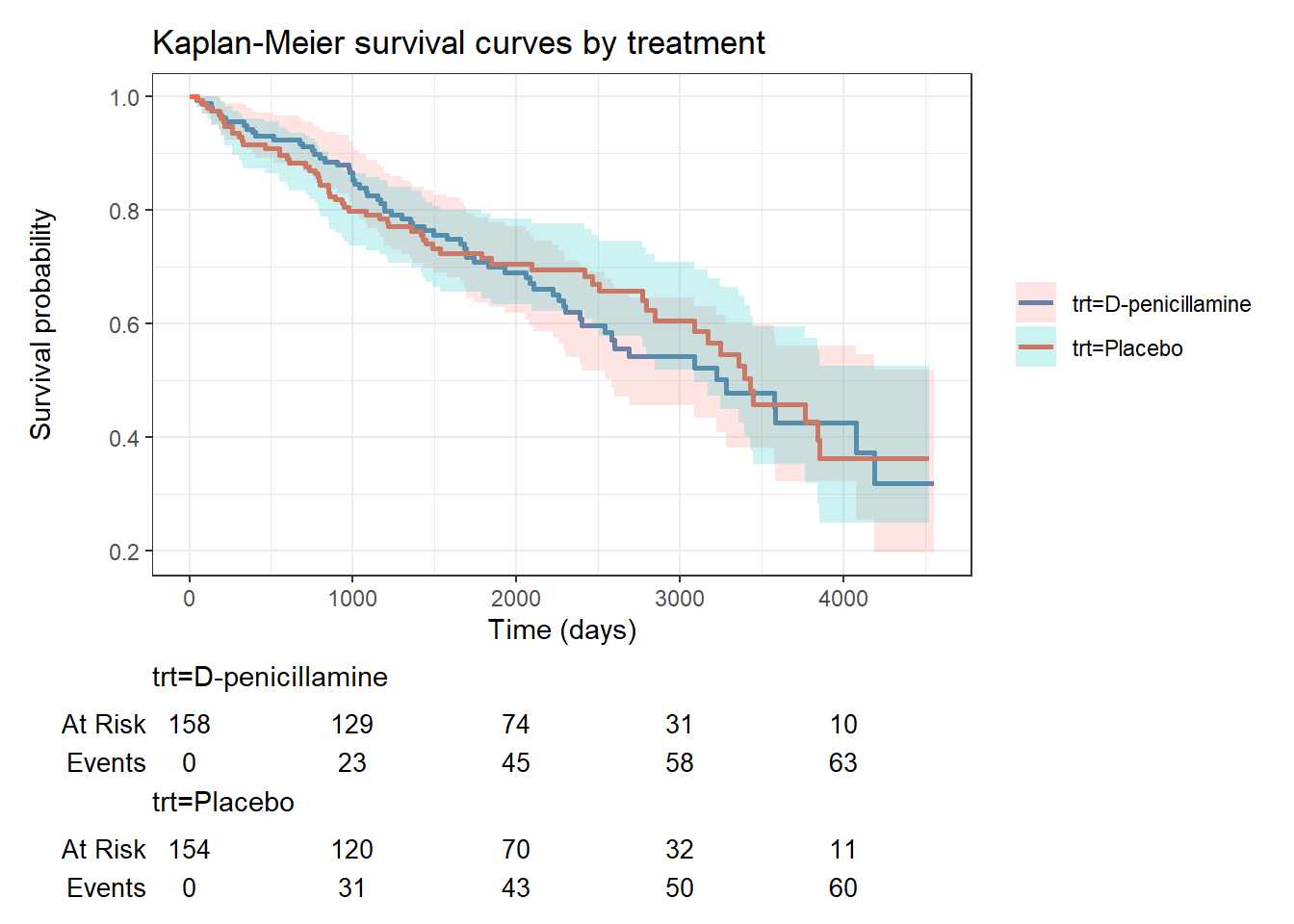
TipRun It Yourself
The two step curves should sit almost on top of each other for the full follow-up period, with heavily overlapping shaded confidence bands. The risk table below the plot shows both groups starting at a similar size (158 vs 154) and losing patients to events at a similar pace (e.g., by day 2920, 58 of 158 D-penicillamine patients and 50 of 154 placebo patients have had the event). Visually, this is what “no treatment effect” looks like.
17.5.3 Log-Rank Test
Estimated time: ~5 minutes (Walkthrough)
survdiff(Surv(time, died) ~ trt, data = pbc)Call:
survdiff(formula = Surv(time, died) ~ trt, data = pbc)
N Observed Expected (O-E)^2/E (O-E)^2/V
trt=D-penicillamine 158 65 63.2 0.0502 0.102
trt=Placebo 154 60 61.8 0.0513 0.102
Chisq= 0.1 on 1 degrees of freedom, p= 0.7
TipRun It Yourself
You should get Chisq = 0.1 on 1 df, p = 0.7. With 65 observed deaths in the D-penicillamine group against 63.2 expected, and 60 observed against 61.8 expected in the placebo group, the data are entirely consistent with no difference between groups. This matches the original PBC trial finding: D-penicillamine showed no survival benefit over placebo.
The log-rank test compares survival curves between groups. A significant p-value means survival differs at some point over follow-up; it does not tell you where or by how much.
17.5.4 Estimating Median Survival
Estimated time: ~5 minutes (Walkthrough)
km_trtCall: survfit(formula = Surv(time, died) ~ trt, data = pbc)
n events median 0.95LCL 0.95UCL
trt=D-penicillamine 158 65 3282 2583 NA
trt=Placebo 154 60 3428 3090 NA
TipRun It Yourself
You should see median survival of 3282 days (95% CI: 2583–NA) for D-penicillamine and 3428 days (95% CI: 3090–NA) for Placebo – about 9 years in both groups, with overlapping confidence intervals (consistent with the log-rank result above). The upper CI is NA for both groups because the survival curve never drops back down to the lower bound needed to compute it within the follow-up period: not every quantity you might want is always estimable from the available data.
The median survival is the time at which \(S(t) = 0.5\). If the curve does not drop below 0.5, the median is not reached within the study period.
17.5.5 Cox Proportional Hazards Model
17.5.5.1 Univariable Cox Models
Estimated time: ~10 minutes (Walkthrough)
cox1 <- coxph(Surv(time, died) ~ trt,      data = pbc)
cox2 <- coxph(Surv(time, died) ~ log_bili, data = pbc)
cox3 <- coxph(Surv(time, died) ~ albumin,  data = pbc)

bind_rows(
  tidy(cox1, conf.int = TRUE, exponentiate = TRUE),
  tidy(cox2, conf.int = TRUE, exponentiate = TRUE),
  tidy(cox3, conf.int = TRUE, exponentiate = TRUE)
) %>%
  select(term, estimate, conf.low, conf.high, p.value)
# A tibble: 3 × 5
term estimate conf.low conf.high p.value
<chr> <dbl> <dbl> <dbl> <dbl>
1 trtPlacebo 0.944 0.665 1.34 7.49e- 1
2 log_bili 2.96 2.47 3.55 2.99e-31
3 albumin 0.166 0.110 0.250 9.85e-18
TipRun It Yourself
You should get a 3-row tibble:
| term | HR | 95% CI | p-value |
|---|---|---|---|
| trtPlacebo | 0.944 | 0.665–1.34 | 0.749 |
| log_bili | 2.96 | 2.47–3.55 | 2.99e-31 |
| albumin | 0.166 | 0.110–0.250 | 9.85e-18 |
trtPlacebo’s HR is close to 1 with a wide, non-significant CI – the Cox model agrees with the log-rank test that treatment has essentially no effect. log_bili and albumin, by contrast, have astronomically small p-values: each is, on its own, a very strong predictor of mortality. This is expected – bilirubin and albumin are direct markers of liver function.
17.5.5.2 Multivariable Cox Model
Estimated time: ~15 minutes (Walkthrough)
cox_full <- coxph(
  Surv(time, died) ~ trt + log_bili + albumin + log_proto + stage,
  data = pbc
)
tidy(cox_full, conf.int = TRUE, exponentiate = TRUE) %>%
  select(term, estimate, conf.low, conf.high, p.value) %>%
  mutate(across(where(is.numeric), \(x) round(x, 3)))
# A tibble: 7 × 5
term estimate conf.low conf.high p.value
<chr> <dbl> <dbl> <dbl> <dbl>
1 trtPlacebo 0.994 0.696 1.42 0.975
2 log_bili 2.30 1.88 2.82 0
3 albumin 0.365 0.23 0.581 0
4 log_proto 48.6 5.27 448. 0.001
5 stageStage 2 4.34 0.559 33.7 0.16
6 stageStage 3 5.49 0.739 40.8 0.096
7 stageStage 4 7.03 0.947 52.1 0.057glance(cox_full)# A tibble: 1 × 18
n nevent statistic.log p.value.log statistic.sc p.value.sc statistic.wald
<int> <dbl> <dbl> <dbl> <dbl> <dbl> <dbl>
1 312 125 186. 1.04e-36 222. 2.56e-44 176
# ℹ 11 more variables: p.value.wald <dbl>, statistic.robust <dbl>,
# p.value.robust <dbl>, r.squared <dbl>, r.squared.max <dbl>,
# concordance <dbl>, std.error.concordance <dbl>, logLik <dbl>, AIC <dbl>,
# BIC <dbl>, nobs <dbl>
TipRun It Yourself
The cox_full table should have 7 rows:
| term | HR | 95% CI | p-value |
|---|---|---|---|
| trtPlacebo | 0.994 | 0.696–1.42 | 0.975 |
| log_bili | 2.30 | 1.88–2.82 | <0.001 |
| albumin | 0.365 | 0.23–0.581 | <0.001 |
| log_proto | 48.6 | 5.27–448 | 0.001 |
| stageStage 2 | 4.34 | 0.559–33.7 | 0.16 |
| stageStage 3 | 5.49 | 0.739–40.8 | 0.096 |
| stageStage 4 | 7.03 | 0.947–52.1 | 0.057 |
glance(cox_full) should report n = 312, nevent = 125, concordance ≈ 0.837, AIC ≈ 1108. A concordance of 0.84 means the model ranks pairs of patients by predicted risk correctly about 84% of the time – a strong model by clinical standards.
Interpreting hazard ratios:
- trt:
trtPlacebohas HR = 0.994 (95% CI 0.696–1.42, p = 0.975) – still indistinguishable from 1 once bilirubin, albumin, prothrombin time, and stage are accounted for. Treatment assignment adds nothing once disease severity is in the model, consistent with the log-rank test and univariable models above. - log_bili: HR = 2.30 (95% CI 1.88–2.82, p < 0.001). Each one-unit increase in log(bilirubin) – a roughly 2.7-fold increase in bilirubin on the original scale – multiplies the hazard of death by about 2.3, i.e. a 130% higher hazard, after adjusting for the other predictors.
- albumin: HR = 0.365 (95% CI 0.23–0.581, p < 0.001). Each 1 g/dL increase in albumin is associated with a 63.5% lower hazard (HR < 1, protective), after adjustment.
- log_proto: HR = 48.6 (95% CI 5.27–448, p = 0.001). This HR looks enormous, but
protime(prothrombin time) varies over a very narrow range in this data, so a full one-unit change inlog_protorepresents a large relative change in clotting time. Large HRs for log-transformed lab values with a narrow range are common – always check the range of the original variable before reacting to the size of the HR. - stageStage 4: HR = 7.03 (95% CI 0.947–52.1, p = 0.057). The point estimate suggests roughly 7 times the hazard of Stage 1 patients after adjustment, but the confidence interval includes 1 and the p-value sits just above the conventional 0.05 threshold. With only 16 Stage 1 patients (and just 1 death among them), this comparison is imprecise – “not quite significant” here reflects limited data for Stage 1 as much as a weak effect.
Note that the HR is not the same as an odds ratio or a relative risk. See the Logistic Regression session for the OR comparison.
17.5.6 Checking the Proportional Hazards Assumption
Estimated time: ~10 minutes (Walkthrough)
ph_test <- cox.zph(cox_full)
print(ph_test)
chisq df p
trt 1.598 1 0.206
log_bili 0.657 1 0.417
albumin 2.588 1 0.108
log_proto 5.504 1 0.019
stage 8.276 3 0.041
GLOBAL 14.413 7 0.044# These plots use base R since there is no standard ggplot equivalent
# for Schoenfeld residual plots without additional packages
par(mfrow = c(2, 3))
plot(ph_test)
par(mfrow = c(1, 1))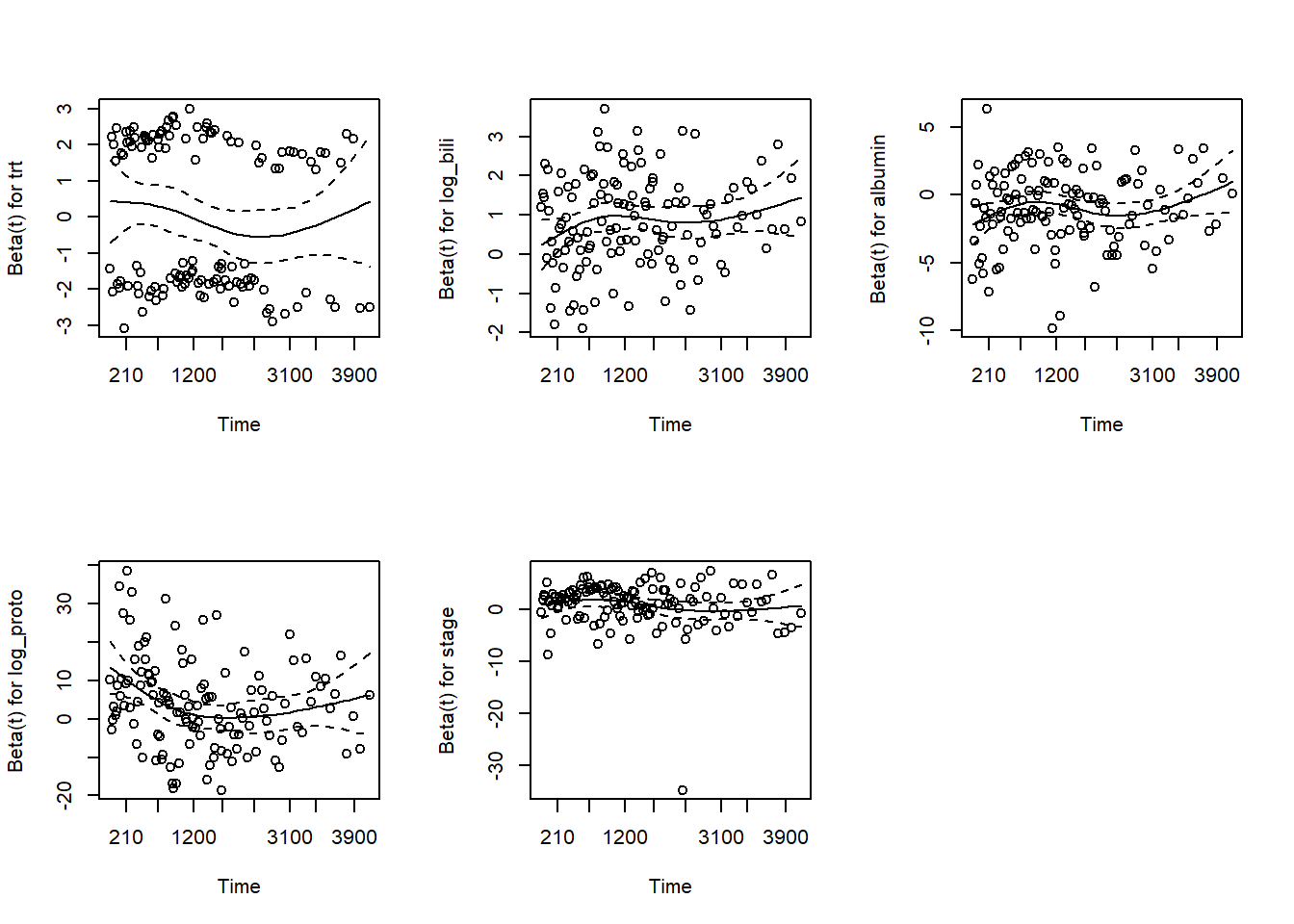
TipRun It Yourself
You should see:
| term | chisq | df | p |
|---|---|---|---|
| trt | 1.598 | 1 | 0.206 |
| log_bili | 0.657 | 1 | 0.417 |
| albumin | 2.588 | 1 | 0.108 |
| log_proto | 5.504 | 1 | 0.019 |
| stage | 8.276 | 3 | 0.041 |
| GLOBAL | 14.413 | 7 | 0.044 |
The GLOBAL test is significant (p = 0.044): the proportional hazards assumption does not hold perfectly for cox_full. log_proto (p = 0.019) and stage (p = 0.041) are the terms driving this. In the Schoenfeld residual plots, the log_proto panel shows a downward-sloping smooth line (its effect on the hazard weakens at later follow-up times), and the stage panel similarly slopes down, with one large outlier point. The other three terms (trt, log_bili, albumin) have roughly flat smooths and non-significant tests – their hazard ratios are reasonably constant over time.
A significant p-value for a term indicates the hazard ratio for that variable changes over time (non-proportional hazards). Here, the global test and the log_proto and stage terms suggest the model would benefit from one of the following:
- Stratification:
coxph(... + strata(stage), ...): allows separate baseline hazards by stage, not estimating a stage HR - Time-varying coefficients:
tt()incoxph - Restricted mean survival time as an alternative summary measure
In practice, a single borderline term in a 5-predictor model followed for over a decade is not unusual, and many analysts would still report cox_full while noting this limitation – but you should always report whether you checked, and what you found.
17.6 Example 2: Melanoma Data
Estimated time: ~20 minutes (Walkthrough)
NoteTeacher Note
Ulceration of a melanoma – the surface of the tumour breaking down – is a well-established marker of aggressive disease. Before running mel-survival, ask learners to predict roughly how different the two KM curves will look, and whether the difference will be larger or smaller than the treatment-effect (non-)difference seen in Example 1. (It is much larger: this is a real prognostic factor, not a null result.)
mel <- boot::melanoma %>%
  as_tibble() %>%
  mutate(
    died_mel   = as.integer(status == 1),
    ulceration = factor(ulcer, levels = c(0, 1), labels = c("No", "Yes")),
    sex        = factor(sex,   levels = c(0, 1), labels = c("Female", "Male")),
    log_thick  = log(thickness)
  )

km_ulc <- survfit(Surv(time, died_mel) ~ ulceration, data = mel)

km_ulc %>%
  ggsurvfit(linewidth = 1) +
  add_confidence_interval() +
  add_risktable() +
  scale_colour_manual(values = c("steelblue", "tomato")) +
  labs(title = "Melanoma survival by ulceration status",
       x = "Time (days)", y = "Survival probability") +
  theme_bw()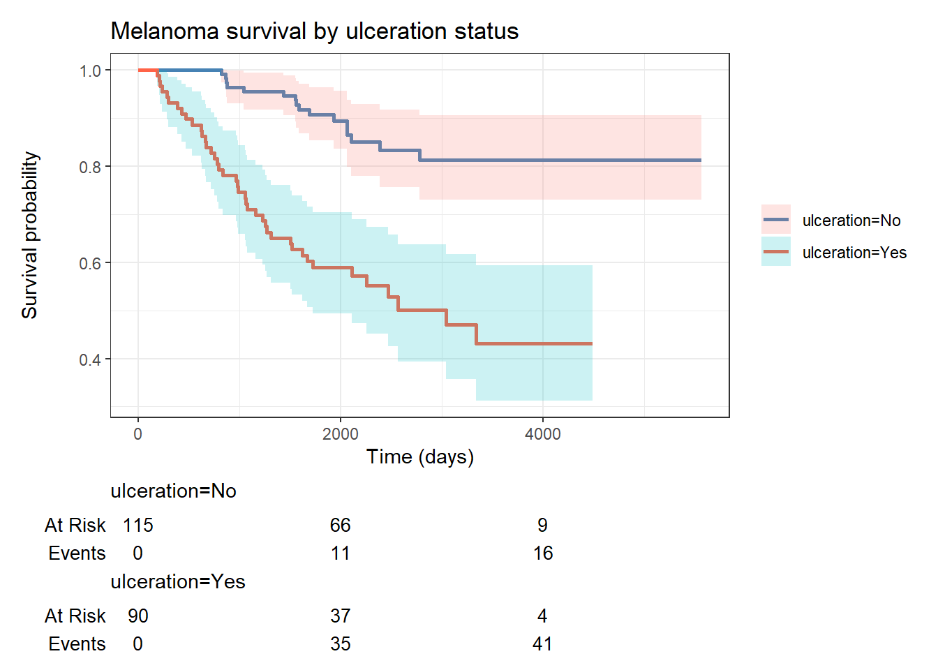
TipRun It Yourself
The two curves should now separate clearly, unlike Example 1. The ulceration = No group (115 patients) stays near 1.0 for the first ~800 days, then declines gently to about 0.81 by the end of follow-up (16 events). The ulceration = Yes group (90 patients) starts declining almost immediately and drops to about 0.43 (41 events) – a much steeper curve with a wider confidence band, reflecting both the higher event rate and the smaller group size. This is what a real prognostic effect looks like next to the null result from Example 1.
cox_mel <- coxph(Surv(time, died_mel) ~ log_thick + ulceration + sex, data = mel)
tidy(cox_mel, conf.int = TRUE, exponentiate = TRUE) %>%
  select(term, estimate, conf.low, conf.high, p.value)
# A tibble: 3 × 5
term estimate conf.low conf.high p.value
<chr> <dbl> <dbl> <dbl> <dbl>
1 log_thick 1.78 1.25 2.53 0.00133
2 ulcerationYes 2.56 1.35 4.83 0.00379
3 sexMale 1.46 0.862 2.49 0.159
TipRun It Yourself
You should get a 3-row tibble:
| term | HR | 95% CI | p-value |
|---|---|---|---|
| log_thick | 1.78 | 1.25–2.53 | 0.00133 |
| ulcerationYes | 2.56 | 1.35–4.83 | 0.00379 |
| sexMale | 1.46 | 0.862–2.49 | 0.159 |
Both log_thick (each unit increase in log(tumour thickness) more than doubles the hazard… well, multiplies it by 1.78) and ulcerationYes (an ulcerated tumour roughly 2.6 times the hazard of a non-ulcerated one of the same thickness and sex) are significant after mutual adjustment. sexMale has HR > 1 (men have higher point-estimate risk) but the CI crosses 1 – not significant here, though sex differences in melanoma outcomes are reported elsewhere in the literature with larger samples.
NoteWhere to Find Data Like This
survival::pbc: 418 PBC patients with time-to-transplant/death, multiple clinical covariates, the primary teaching dataset for this session.
survival::lung: Lung cancer patients with ECOG performance scores, commonly used for Cox model examples.
boot::melanoma: 205 melanoma patients with thickness, ulceration, and survival time.
survival::ovarian, survival::veteran: Further classic teaching datasets in the survival package.
WarningWhat Can Go Wrong
Estimated time: ~10 minutes (Reading)
Ignoring censoring (using logistic or linear regression). Using a binary “died/alive” outcome discards timing information and biases estimates when follow-up lengths differ. Always use time-to-event methods when censoring is present.
Assuming proportional hazards without checking. Cox models assume constant hazard ratios over time. If treatment benefit wanes or emerges late, HRs averaged over the whole follow-up are misleading. Always run cox.zph().
Immortal time bias. If covariates are recorded after study entry (e.g., “did the patient receive surgery?”), misclassifying the period before surgery as exposed creates an artificial survival advantage. Use landmark analysis or time-varying covariates to address this.
Competing risks. If patients can die from liver disease or be transplanted, transplant is a competing risk for death. Treating transplant as censoring overestimates the probability of disease death. Use the cmprsk or tidycmprsk package for competing risks analysis.
17.7 Exercises
NoteTeacher Note
Before Exercise 1, ask learners to predict: with 312 patients split across 4 disease stages (16 / 67 / 120 / 109), and stage being a strong predictor in cox_full, will the log-rank test across all 4 stages be significant – and if so, how significant compared to the trt comparison (p = 0.7)? (It is dramatically more significant: p ≈ 1e-11.) Exercise 2 also revisits the proportional-hazards theme from Example 1 – another model, another borderline PH violation.
17.7.1 Exercise 1 (Guided): KM Curves by Disease Stage
Estimated time: ~15 minutes (Practice)
Using pbc, plot Kaplan-Meier survival curves separately for each disease stage. Use add_risktable(). Then run the log-rank test.
TipExercise 1: Solution
km_stage <- survfit(Surv(time, died) ~ stage, data = pbc)

km_stage %>%
  ggsurvfit(linewidth = 0.8) +
  add_confidence_interval(alpha = 0.15) +
  add_risktable() +
  labs(title = "Survival by disease stage",
       x = "Time (days)", y = "Survival probability") +
  theme_bw()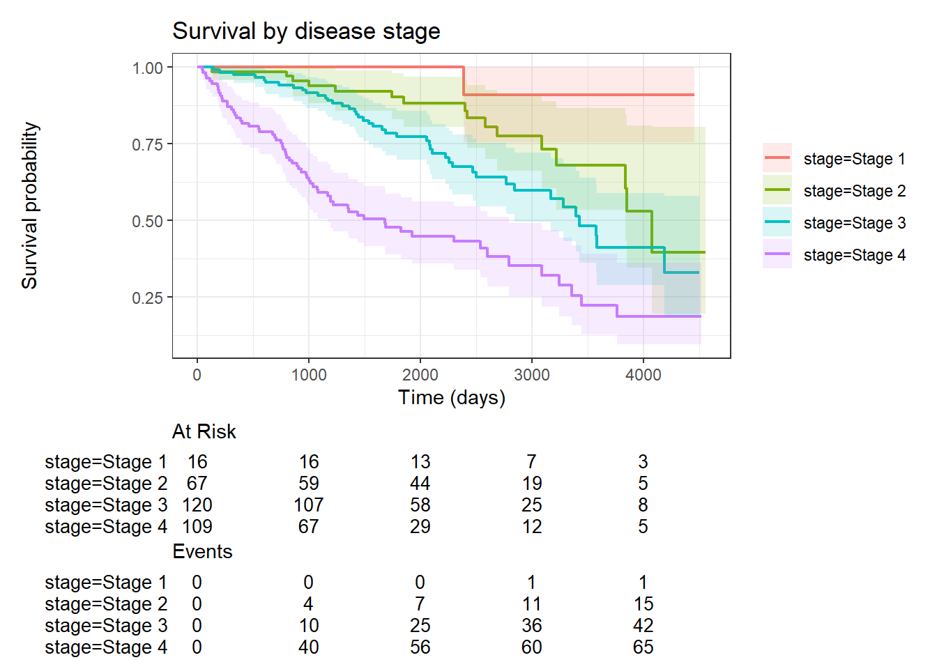
survdiff(Surv(time, died) ~ stage, data = pbc)Call:
survdiff(formula = Surv(time, died) ~ stage, data = pbc)
N Observed Expected (O-E)^2/E (O-E)^2/V
stage=Stage 1 16 1 9.9 8.00 8.78
stage=Stage 2 67 16 32.3 8.22 11.17
stage=Stage 3 120 43 51.2 1.30 2.22
stage=Stage 4 109 65 31.6 35.17 47.84
Chisq= 53.8 on 3 degrees of freedom, p= 1e-11 The four curves should fan out clearly, with Stage 1 staying near 1.0 throughout and Stage 4 dropping to around 0.2 by the end of follow-up. The log-rank test gives Chisq = 53.8 on 3 df, p = 1e-11 – overwhelmingly significant, in sharp contrast to the trt comparison (Chisq = 0.1, p = 0.7). The per-stage observed-vs-expected counts show why: Stage 1 had only 1 death against 9.9 expected, while Stage 4 had 65 against 31.6 expected. Disease stage, unlike treatment, is a real and large driver of survival differences.
17.7.2 Exercise 2 (Semi-guided): Adjusted Cox Model for Melanoma
Estimated time: ~20 minutes (Practice)
Using boot::melanoma:
- Fit a univariable Cox model for
log_thick. - Add
ulceration. How does the HR for thickness change? - Add
sex. Compare AIC. - Check proportional hazards with
cox.zph(). Is any variable problematic?
TipExercise 2: Solution
m1 <- coxph(Surv(time, died_mel) ~ log_thick,              data = mel)
m2 <- coxph(Surv(time, died_mel) ~ log_thick + ulceration, data = mel)
m3 <- coxph(Surv(time, died_mel) ~ log_thick + ulceration + sex, data = mel)

bind_rows(
  tidy(m1, exponentiate = TRUE) %>% mutate(model = "1: thickness"),
  tidy(m2, exponentiate = TRUE) %>% mutate(model = "2: + ulceration"),
  tidy(m3, exponentiate = TRUE) %>% mutate(model = "3: + sex")
) %>%
  filter(term == "log_thick") %>%
  select(model, estimate, p.value)
# A tibble: 3 × 3
model estimate p.value
<chr> <dbl> <dbl>
1 1: thickness 2.28 0.000000107
2 2: + ulceration 1.84 0.000520
3 3: + sex 1.78 0.00133 AIC(m1, m2, m3) df AIC
m1 1 537.8406
m2 2 529.7198
m3 3 529.7398cox.zph(m3) chisq df p
log_thick 6.96 1 0.0083
ulceration 3.65 1 0.0560
sex 1.20 1 0.2728
GLOBAL 7.99 3 0.0461The log_thick HR drops from 2.28 (model 1, p ≈ 1.07e-7) to 1.84 (model 2, p = 0.00052) once ulceration is added – thickness and ulceration are correlated (thicker tumours are more likely to be ulcerated), so part of what looked like a thickness effect was really an ulceration effect. Adding sex barely moves it further, to 1.78 (model 3, p = 0.00133).
AIC(m1, m2, m3) gives 537.84, 529.72, 529.74 for models 1–3: adding ulceration improves the model by about 8 AIC points, but adding sex on top makes essentially no difference (529.72 vs 529.74) – model 2 is the most parsimonious adequate model.
cox.zph(m3) gives log_thick chisq = 6.96, p = 0.0083; ulceration p = 0.056; sex p = 0.273; GLOBAL p = 0.046. Just as with cox_full in Example 1, the proportional hazards assumption is not perfectly satisfied here either – log_thick’s effect appears to weaken at later times. This is a second example of the same realistic pattern: significant predictors whose hazard ratios are not perfectly constant over a long follow-up.
17.7.3 Exercise 3 (Open-ended)
Estimated time: 15–30 minutes (Practice)
Using survival::lung, fit a multivariable Cox model predicting death from ECOG performance score, age, sex, and weight loss. Check proportional hazards. Write a Results paragraph reporting HRs with 95% CIs for each predictor, as you would in a clinical paper. Include a KM plot stratified by ECOG category.
17.8 Comprehension Check
Estimated time: ~10 minutes (Self-test)
- A patient is censored at 800 days with
died = 0. What does this mean, and how does the Cox model use this data point? - You compare two KM curves with the log-rank test and get p = 0.04. What exactly is being tested?
- In
cox_full, the HR for log_bili is 2.30 (95% CI 1.88–2.82). Interpret this in plain language. - In
cox_full,cox.zph()gives p = 0.041 for stage (and a GLOBAL p = 0.044). What is the problem, and what are your options? - Your study has 200 patients, of whom 120 were transplanted before dying. Why is treating transplant as censoring a problem?
NoteAnswers
- The patient was alive at 800 days when observation ended, whether by end of study, loss to follow-up, or administrative censoring. The Cox model uses this as a partial likelihood contribution: the patient was in the risk set at all times up to 800 days and did not have the event. Their data provides information about who was at risk but does not contribute a completed failure time.
- The log-rank test evaluates the null hypothesis that the two survival curves are identical over the entire follow-up period: expected and observed numbers of deaths are equal across all time points. p = 0.04 means the evidence against identical survival curves reaches conventional significance. It does not specify where the curves diverge or by how much.
- Each 2.72-fold increase in bilirubin (one unit on the log scale) is associated with a 2.30-times higher instantaneous rate of dying (hazard), after adjustment for the other variables in the model (treatment, albumin, prothrombin time, and disease stage). Patients with bilirubin 2.72 times higher are estimated to die at roughly 2.3 times the rate of otherwise similar patients – this is the actual
cox_fullresult computed earlier in this session. - The proportional hazards assumption is violated for stage (and, with a GLOBAL p = 0.044, for the model overall); the hazard ratio between stages is not constant over time. Options: (1) stratify by stage using
strata(stage), which allows separate baseline hazards per stage but does not estimate a stage HR; (2) include astage:log(time)interaction term to model the time-varying hazard ratio; (3) use restricted mean survival time (RMST) as an alternative summary that does not assume proportionality. - Transplant is a competing risk for death from liver disease; a patient who receives a transplant can no longer die from the disease. Treating transplant as censoring falsely assumes these patients had the same underlying risk as uncensored patients, which overestimates the cumulative incidence of disease-specific death. The correct analysis uses cumulative incidence functions and the Fine-Gray or cause-specific Cox model.
17.9 How to Report
Note
In a methods section: “Time-to-event data were analysed using the Kaplan-Meier estimator and log-rank test to compare survival between groups. Cox proportional hazards regression was used to estimate hazard ratios adjusted for [covariates]. The proportional hazards assumption was assessed using Schoenfeld residuals.”
In results (Kaplan-Meier): “Median survival was X months (95% CI [L, U]) in [group A] and Y months (95% CI [L, U]) in [group B] (log-rank p = Z). The 1-year survival probability was X% (95% CI [L, U]) in [group A].”
In results (Cox model): “[Predictor] was significantly associated with mortality after adjustment for [covariates] (HR = X, 95% CI [L, U], p = Y).”
Always include:
- Median survival with 95% CI for each group
- Number of events and total observations (e.g., “87 deaths in 312 patients, median follow-up 4.2 years”)
- Hazard ratio with 95% CI (not odds ratio)
- Confirmation that the proportional hazards assumption was assessed
HR ≠ RR: The hazard ratio approximates the relative risk only when events are rare and follow-up is short. Never describe an HR as a “relative risk” in a survival context.
17.10 Further Reading
- Therneau and Grambsch (2000): Modeling Survival Data: Extending the Cox Model
vignette("survival", package = "survival"): comprehensive package vignetteggsurvfitpackage documentation for publication-quality KM plots- Royston and Lambert (2011): Restricted mean survival time: an alternative to the hazard ratio (Statistics in Medicine)
Royston, Patrick, and Paul C. Lambert. 2011. Flexible Parametric Survival Analysis Using Stata: Beyond the Cox Model. Stata Press.
Therneau, Terry M., and Patricia M. Grambsch. 2000. Modeling Survival Data: Extending the Cox Model. Springer.