set.seed(2024)
n <- 5000

# Simulate genetic score (standardised polygenic score for LDL)
G <- rbinom(n, 2, 0.3)          # 0/1/2 copies of effect allele

# Simulate confounder (BMI) - NOT associated with G (by Mendel's laws)
BMI <- rnorm(n, 25, 4)

# LDL causally affected by G and BMI
LDL <- 0.8 * G + 0.4 * BMI + rnorm(n, 0, 1.5)

# ALT: true causal effect of LDL = 0.3; also affected by BMI (confounder)
ALT <- 0.3 * LDL + 0.5 * BMI + rnorm(n, 0, 2)

sim <- tibble(G, BMI, LDL, ALT)19 Mendelian Randomisation
NoteSession at a Glance
Total core time: ~145 minutes (about 2.5 hours). A natural break point is after Example 1 (the simulated one-sample MR analysis)—cover Example 2 (two-sample MR) and the exercises in a second sitting. Exercise 3 is open-ended and its time will vary.
| Section | Time | Type |
|---|---|---|
| The Key Idea: Nature’s Randomised Trial | ~10 min | Concept |
| Background: MR as an Instrument | ~15 min | Concept |
| Example 1: Simulated One-Sample MR | ~30 min | Walkthrough |
| Example 2: Summary-Level Two-Sample MR | ~20 min | Walkthrough |
| What Can Go Wrong | ~10 min | Reading |
| Exercise 1 (Guided) | ~15 min | Practice |
| Exercise 2 (Semi-guided) | ~15 min | Practice |
| Exercise 3 (Open-ended) | 15–30 min | Practice |
| Comprehension Check | ~10 min | Self-test |
If you are short on time, focus on Example 1’s naive-ols and wald-ratio chunks: they show, side by side, how a confounded OLS estimate (0.906, more than triple the true effect) and an MR estimate (0.345, close to the true effect of 0.3) can disagree dramatically for the same simulated data.
TipHow to Use the Code in This Session
Every code chunk below is written so you can copy it into your R console (or an R script) and run it yourself, in the order shown. Where you see a “Run It Yourself” box, stop and run the code above it before reading the explanation that follows.
19.1 When Do You Use This?
Tip
You want to know whether high LDL cholesterol causally increases the risk of liver disease. Observational studies are confounded: sick people may both have elevated LDL and worse liver function. An RCT randomising people to high or low LDL is impossible. Mendelian randomisation uses genetic variants that naturally raise LDL as a randomisation instrument: because genotype is assigned at conception, it cannot be confounded by lifestyle or disease state.
NoteTeacher Note
Before going further, ask learners: if LDL and a liver enzyme (ALT) are both raised by a common factor (say, BMI), what would you expect a simple lm(ALT ~ LDL) regression to show, compared to the true causal effect of LDL on ALT? Will the OLS estimate be too high, too low, or about right? Keep this prediction in mind for Example 1, where both numbers are computed directly.
19.2 Learning Objectives
After completing this session you will be able to:
- Explain the IV/MR framework and the three core instrument assumptions
- Simulate MR data and estimate a causal effect with the Wald ratio and two-stage least squares (2SLS)
- Apply MR with summary-level GWAS data using the
TwoSampleMRpackage - Interpret MR effect estimates and report them correctly
- Recognise horizontal pleiotropy and apply sensitivity analyses (MR-Egger, weighted median, MR-PRESSO)
19.3 The Key Idea: Nature’s Randomised Trial
Estimated time: ~10 minutes (Concept)
Randomisation is the gold standard for establishing causation because it breaks the link between who receives treatment and everything else about those people. In an RCT, you randomly assign some people to high LDL (or a drug that raises LDL) and compare their outcomes to a control group.
Mendelian randomisation says: nature has already done this. Genetic variants that raise LDL are distributed essentially at random in the population (by Mendel’s laws of segregation). People who inherited more LDL-raising alleles are, on average, no different from those who inherited fewer, except for their LDL level. So we can use the genetic “dose” as a proxy for random assignment to high or low LDL.
The key difference from an RCT: you cannot verify the assumptions as directly. This is why sensitivity analyses for pleiotropy are essential; see the Causal Inference session for the broader framework.
19.4 Background: Mendelian Randomisation as an Instrument
Estimated time: ~15 minutes (Concept)
19.4.1 The Instrumental Variable Framework
An instrumental variable (IV) \(Z\) satisfies three assumptions:
| Assumption | Condition | How to check |
|---|---|---|
| Relevance | \(Z\) is associated with the exposure \(X\) | F-statistic > 10 in first stage |
| Independence (exchangeability) | \(Z\) is not associated with confounders \(U\) | By Mendel’s laws: genes assigned randomly at meiosis |
| Exclusion restriction | \(Z\) affects the outcome \(Y\) only through \(X\) | Untestable; violated by horizontal pleiotropy |
In MR, the IV is a genetic variant (SNP) associated with the exposure. Because genotype is determined before disease and is largely orthogonal to environmental confounders, it approximates a natural randomisation.
19.4.2 The Wald Ratio Estimator
With a single SNP instrument:
\[\hat{\beta}_{MR} = \frac{\hat{\beta}_{ZY}}{\hat{\beta}_{ZX}}\]
where \(\hat{\beta}_{ZY}\) is the SNP-outcome association and \(\hat{\beta}_{ZX}\) is the SNP-exposure association. Both are obtained from GWAS summary statistics (or individual-level regression in one-sample MR).
19.5 Example 1: Simulated One-Sample MR
Estimated time: ~30 minutes (Walkthrough)
NoteTeacher Note
This example has the data-generating process spelled out in code (simulate-mr), so the “true” causal effect (0.3) is known by construction - a luxury we never have with real data. Use this to make predictions concrete:
- Before running
naive-ols: ask learners to predict whether the naivelm(ALT ~ LDL)estimate will be above, below, or equal to 0.3, and why (BMI raises both LDL and ALT). - Before running
wald-ratio: ask learners to predict whether the genetic-instrument-based estimate will be closer to 0.3 than the OLS estimate, and why genotypeGis not affected by BMI.
We simulate a dataset where LDL causally increases liver enzyme (ALT), with confounding by BMI.
19.5.1 Naive OLS (confounded)
Estimated time: ~5 minutes (Walkthrough)
# OLS is biased because BMI confounds LDL-ALT association
fit_ols <- lm(ALT ~ LDL, data = sim)
tidy(fit_ols, conf.int = TRUE) %>% filter(term == "LDL")
# A tibble: 1 × 7
term estimate std.error statistic p.value conf.low conf.high
<chr> <dbl> <dbl> <dbl> <dbl> <dbl> <dbl>
1 LDL 0.906 0.0155 58.6 0 0.876 0.937
TipRun It Yourself
You should see (rounded):
| term | estimate | std.error | statistic | p.value | conf.low | conf.high |
|---|---|---|---|---|---|---|
| LDL | 0.906 | 0.0155 | 58.6 | <0.001 | 0.876 | 0.937 |
The naive OLS estimate (0.906) is roughly three times the true causal effect of 0.3 that we built into the simulation. The confidence interval (0.876, 0.937) does not even come close to containing 0.3. This is exactly the bias predicted in the Teacher Note: BMI raises both LDL and ALT, so part of the LDL-ALT association in this regression reflects their shared dependence on BMI, not a direct causal effect of LDL on ALT.
The OLS estimate is inflated because BMI raises both LDL and ALT.
19.5.2 Wald Ratio MR
Estimated time: ~10 minutes (Walkthrough)
# First stage: SNP - LDL (relevance check)
fit_z_x <- lm(LDL ~ G, data = sim)
beta_zx  <- coef(fit_z_x)["G"]
se_zx    <- summary(fit_z_x)$coefficients["G", "Std. Error"]
f_stat   <- (beta_zx / se_zx)^2
cat("First-stage F-statistic:", round(f_stat, 1), "\n")
First-stage F-statistic: 291.3 # Reduced form: SNP - ALT
fit_z_y <- lm(ALT ~ G, data = sim)
beta_zy <- coef(fit_z_y)["G"]
se_zy <- summary(fit_z_y)$coefficients["G", "Std. Error"]
# Wald ratio
beta_mr <- beta_zy / beta_zx
se_mr <- se_zy / abs(beta_zx) # delta method (approximate)
cat("Wald ratio MR estimate:", round(beta_mr, 3),
"| SE:", round(se_mr, 3),
"| 95% CI: (", round(beta_mr - 1.96 * se_mr, 3), ",",
round(beta_mr + 1.96 * se_mr, 3), ")\n")Wald ratio MR estimate: 0.345 | SE: 0.085 | 95% CI: ( 0.177 , 0.512 )cat("True causal effect: 0.3\n")True causal effect: 0.3
TipRun It Yourself
You should see:
First-stage F-statistic: 291.3
Wald ratio MR estimate: 0.345 | SE: 0.085 | 95% CI: ( 0.177 , 0.512 )
True causal effect: 0.3
Two things to notice:
- The instrument is strong. The first-stage F-statistic (291.3) is far above the rule-of-thumb threshold of 10, so the relevance assumption is well satisfied here -
Gis a good predictor ofLDL. - The MR estimate recovers the true effect. 0.345 (95% CI 0.177 to 0.512) is close to the true causal effect of 0.3, and the CI comfortably contains it - unlike the OLS estimate of 0.906. Because
Gis assigned at conception (by Mendel’s laws) and is not associated withBMIin this simulation, the SNP-outcome association is not contaminated by the BMI confounding that biased the OLS estimate.
19.5.3 Two-Stage Least Squares (2SLS)
Estimated time: ~5 minutes (Walkthrough)
fit_iv <- ivreg(ALT ~ LDL | G, data = sim)
tidy(fit_iv, conf.int = TRUE) %>% filter(term == "LDL")
TipRun It Yourself
This chunk only runs if the AER package is installed (it is skipped otherwise, with a message from the setup chunk). If you have AER available, run it and compare the LDL row to the Wald ratio above: with a single instrument, 2SLS is mathematically equivalent to the Wald ratio, so you should get the same estimate (≈0.345) and a very similar standard error.
2SLS is the multi-instrument generalisation of the Wald ratio. The result should match the Wald ratio when only one instrument is used.
19.6 Example 2: Summary-Level Two-Sample MR
Estimated time: ~20 minutes (Walkthrough)
NoteTeacher Note
The two-sample-mr chunk below is marked eval: false because it queries the live MR-Base/IEU OpenGWAS database over the internet and requires the TwoSampleMR package. It will not run as part of this session, but the code is realistic - if learners have internet access and the package installed, they can run it themselves outside the session to fetch real LDL/CAD summary statistics. The pleiotropy-sim chunk that follows is a self-contained simulation that does run, and illustrates the kind of scatter plot the TwoSampleMR package would produce from real data.
Two-sample MR uses GWAS summary statistics from two independent datasets: - Exposure GWAS: SNP-LDL associations (e.g., from UK Biobank) - Outcome GWAS: SNP-liver disease associations (e.g., FinnGen)
Here we use the TwoSampleMR package to query the MR-Base database.
library(TwoSampleMR)

# Example: LDL - coronary artery disease (publicly available data)
exposure <- extract_instruments("ieu-a-300")     # LDL from GLGC GWAS
outcome  <- extract_outcome_data(
  snps    = exposure$SNP,
  outcomes = "ieu-a-7"                           # CAD from CARDIoGRAM
)
dat <- harmonise_data(exposure, outcome)

# Primary MR methods
res <- mr(dat)
res %>% select(method, b, se, pval, lo_ci, up_ci)
The output reports: - IVW (inverse-variance weighted): Main estimate (assumes no directional pleiotropy) - MR-Egger: Allows for pleiotropy; the intercept tests for it - Weighted median: Consistent estimate if >50% of instruments are valid - MR-PRESSO: Detects and corrects for outlier pleiotropy
19.6.1 Sensitivity Analysis: Pleiotropy
Estimated time: ~10 minutes (Walkthrough)
# Simulated scatter plot: SNP effects on exposure vs outcome
set.seed(42)
n_snps  <- 20
beta_x  <- rnorm(n_snps, 0.05, 0.02)        # SNP-LDL effects
beta_y  <- 0.3 * beta_x + rnorm(n_snps, 0, 0.008)  # SNP-outcome (no pleiotropy)

tibble(beta_x, beta_y) %>%
  ggplot(aes(x = beta_x, y = beta_y)) +
  geom_point(size = 2, colour = "steelblue") +
  geom_smooth(method = "lm", se = TRUE, colour = "tomato") +
  geom_hline(yintercept = 0, linetype = "dashed") +
  labs(title = "MR scatter plot: SNP effects on exposure vs outcome",
       x = "SNP--Exposure (LDL) effect",
       y = "SNP--Outcome (ALT) effect") +
  theme_bw()
`geom_smooth()` using formula = 'y ~ x'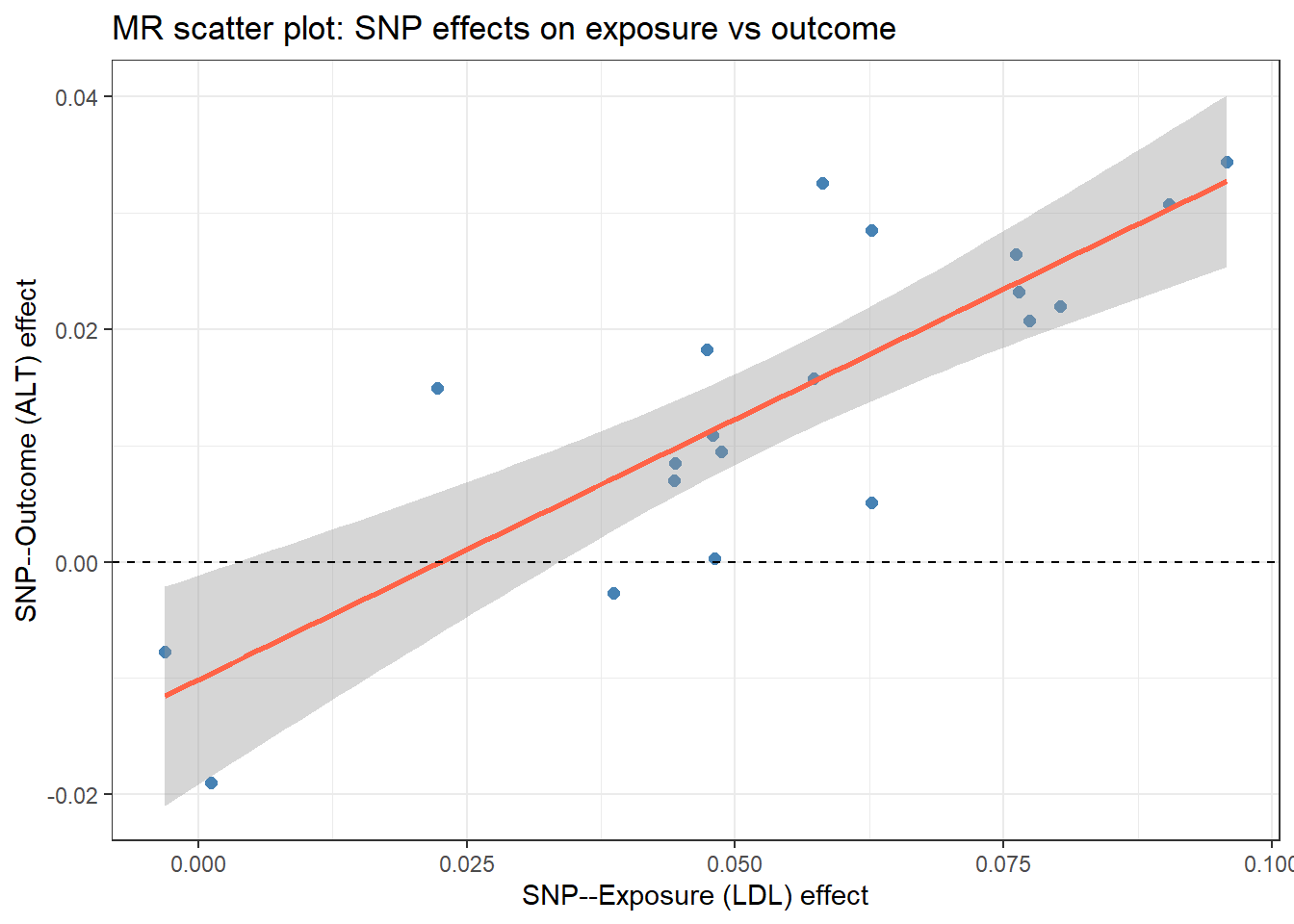
TipRun It Yourself
The plot shows 20 points (one per simulated SNP), with SNP-exposure effects (beta_x) on the x-axis and SNP-outcome effects (beta_y) on the y-axis. The points trend upward from bottom-left to top-right, and the fitted regression line (red) passes close to the origin - near beta_x = 0, the fitted beta_y is close to 0.
This is what an MR-Egger plot looks like when there is no directional pleiotropy: the line’s slope (≈0.3, matching how beta_y was simulated from beta_x) represents the causal effect estimate, and an intercept close to zero means the SNPs’ effects on the outcome are well explained by their effects on the exposure alone - none of them appear to have a “shortcut” direct effect on the outcome. Compare this to Exercise 2, where a SNP with a genuine direct effect on the outcome (horizontal pleiotropy) biases the corresponding estimate.
NoteWhere to Find Data Like This
MR-Base (IEU Open GWAS): TwoSampleMR::available_outcomes(): thousands of GWAS summary datasets freely accessible via the TwoSampleMR package.
UK Biobank GWAS: Downloadable summary statistics for thousands of traits at ukbiobank.ac.uk.
FinnGen: European biobank GWAS summary data at finngen.fi.
PhenoScanner: Query SNP associations across thousands of traits at phenoscanner.medschl.cam.ac.uk.
WarningWhat Can Go Wrong
Estimated time: ~10 minutes (Reading)
Weak instruments (F < 10). When the SNP explains little variance in the exposure, the Wald ratio becomes unstable. Weak instruments bias 2SLS toward the OLS estimate in one-sample MR, and toward the null in two-sample MR. Use multiple SNPs and check F-statistics.
Horizontal pleiotropy. The exclusion restriction is violated if the SNP affects the outcome through pathways other than the exposure. MR-Egger, weighted median, and MR-PRESSO test for and partly correct this, but they are not definitive. Biological understanding of the genetic variant is essential.
Winner’s curse in instrument selection. Using the same dataset to select instruments and to estimate the causal effect inflates the apparent SNP-exposure association. Always use independent datasets for instrument selection and effect estimation (two-sample design).
Confounding by population stratification. If the exposure and outcome GWAS come from populations with different ancestry, SNP effects may differ by ancestry and confound the MR estimate. Use ancestry-matched datasets or multi-ancestry sensitivity analyses.
19.7 Exercises
NoteTeacher Note
Both exercises take the strong instrument from Example 1 (F = 291.3, MR estimate close to the truth) and break one of the IV assumptions on purpose. Exercise 1 breaks relevance (a much weaker SNP-exposure association); Exercise 2 breaks the exclusion restriction (the SNP also has a direct effect on the outcome). Ask learners, before they run either solution, which IV assumption is being violated and what direction of bias they expect.
19.7.1 Exercise 1 (Guided): First-Stage F-Statistic
Estimated time: ~15 minutes (Practice)
Using the simulated sim dataset:
- Regress
LDL ~ Gand compute the F-statistic for the instrument. - What is the rule of thumb? Is your instrument strong?
- Now simulate a weak instrument: replace
GwithG_weak <- rbinom(n, 2, 0.05). Recompute the F-statistic. What changes?
TipExercise 1: Solution
fit1 <- lm(LDL ~ G, data = sim)
f    <- summary(fit1)$fstatistic["value"]
cat("F-statistic:", round(f, 1), "--- strong if > 10\n")
F-statistic: 291.3 --- strong if > 10# Weak instrument
G_weak <- rbinom(nrow(sim), 2, 0.05)
LDL_alt <- 0.1 * G_weak + 0.4 * sim$BMI + rnorm(nrow(sim), 0, 1.5)
fit_weak <- lm(LDL_alt ~ G_weak)
cat("Weak instrument F:", round(summary(fit_weak)$fstatistic["value"], 1), "\n")Weak instrument F: 0.2 You should see:
F-statistic: 291.3 --- strong if > 10
Weak instrument F: 0.2
The original instrument is comfortably strong (F = 291.3 ≫ 10). The weak instrument - constructed with a much rarer effect allele (allele frequency 0.05 instead of 0.3) and a smaller per-allele effect (0.1 instead of 0.8) - has an F-statistic of just 0.2, far below the threshold. With an instrument this weak, the Wald ratio’s denominator (\(\hat{\beta}_{ZX}\)) is estimated so imprecisely that the resulting MR estimate would be highly unstable, with a huge standard error, and in one-sample MR would be biased toward the (confounded) OLS estimate.
19.7.2 Exercise 2 (Semi-guided): Horizontal Pleiotropy Check
Estimated time: ~15 minutes (Practice)
Extend the simulation to add horizontal pleiotropy: the SNP also directly affects ALT (independent of LDL).
- Simulate
ALT_pleiotropic <- 0.3 * LDL + 0.5 * BMI + 0.4 * G + rnorm(n, 0, 2)(direct SNP effect = 0.4). - Compute the Wald ratio MR estimate. Is it biased?
- Interpret: what would this mean in a real MR study?
TipExercise 2: Solution
ALT_p <- 0.3 * sim$LDL + 0.5 * sim$BMI + 0.4 * sim$G + rnorm(nrow(sim), 0, 2)

# SNP-outcome (includes direct path)
beta_zy_p <- coef(lm(ALT_p ~ sim$G))["sim$G"]
wald_p    <- beta_zy_p / beta_zx

cat("True causal effect: 0.3\n")
True causal effect: 0.3cat("Wald ratio with pleiotropy:", round(wald_p, 3), "\n")Wald ratio with pleiotropy: 0.773 # Biased upward because SNP -> ALT directly inflates beta_zyYou should see:
True causal effect: 0.3
Wald ratio with pleiotropy: 0.773
Adding a direct SNP-to-ALT effect of 0.4 (independent of LDL) more than doubles the MR estimate, from a true effect of 0.3 to an apparent 0.773. This is horizontal pleiotropy: the exclusion restriction is violated because the SNP affects the outcome through a pathway other than the exposure (LDL). The Wald ratio attributes the entire SNP-outcome association to the SNP-LDL pathway, so the direct effect gets folded into the causal estimate as bias.
In a real MR study, you would not know the true effect or the size of any direct pathway. This is exactly why sensitivity analyses such as MR-Egger (which can detect a non-zero intercept, as in Comprehension Check Q3) and the weighted median are essential: they provide a way to detect and partially correct for this kind of bias when it cannot be ruled out by design.
19.7.3 Exercise 3 (Open-ended)
Estimated time: 15–30 minutes (Practice)
Identify a trait relevant to your research that has publicly available GWAS summary data (check MR-Base or GWAS Catalog). Design an MR study:
- State your causal hypothesis (exposure → outcome).
- List the MR assumptions and how they might be violated for your chosen instrument.
- Specify which sensitivity analyses you would run and what conclusions you could draw if they disagree with the IVW result.
19.8 Comprehension Check
Estimated time: ~10 minutes (Self-test)
- Why does Mendelian randomisation approximate an RCT?
- The F-statistic for your genetic instrument is 7.2. What is the concern, and what should you do?
- MR-Egger gives a non-zero intercept (p = 0.02). What does this mean?
- The IVW MR estimate is 0.4 but the weighted median estimate is 0.1. How should you interpret this discrepancy?
- Your exposure and outcome GWAS come from the same cohort. What problem does this introduce?
NoteAnswers
- Genetic variants are assigned at conception by the random process of meiosis, effectively a natural randomisation that is independent of most environmental confounders, reverse causation (genes precede disease), and confounders that develop over the life course. This mimics the randomised assignment in an RCT, though only for the specific exposure pathway affected by those variants.
- F < 10 indicates a weak instrument. Weak instruments lead to inflated standard errors, low power, and in one-sample MR, bias toward the OLS estimate. Options: add more SNPs to construct a stronger polygenic score, or restrict to SNPs from larger GWAS with better power. Do not proceed with MR if the instrument is too weak.
- A significant MR-Egger intercept means that the SNP effects on the outcome have a direction-dependent offset after regressing on SNP-exposure effects, evidence of directional (systematic) horizontal pleiotropy. The IVW estimate is biased. The MR-Egger slope provides a pleiotropy-corrected estimate, but it is less precise than IVW.
- The IVW assumes all instruments are valid; if some SNPs are pleiotropic, the IVW is biased. The weighted median is consistent if at least 50% of the instrument weight comes from valid SNPs. A large discrepancy (0.4 vs 0.1) suggests substantial pleiotropy. Report all estimates, run MR-PRESSO to identify outlier SNPs, and interpret cautiously. The true causal effect is probably closer to the more conservative weighted-median estimate.
- This is the one-sample overlap problem. When instrument selection and causal estimation use the same dataset, the winner’s curse inflates the apparent instrument strength, and the 2SLS estimate is biased toward the OLS (confounded) estimate in proportion to the instrument’s weakness. A two-sample design - instrument-exposure association from one independent GWAS, instrument-outcome association from another - avoids this.
19.9 How to Report
19.9.1 Reporting Mendelian Randomisation Results
Note
In a methods section: “Two-sample Mendelian randomisation was performed using summary-level GWAS data for [exposure] (source: [citation]) and [outcome] (source: [citation]). The primary analysis used the inverse-variance weighted (IVW) method. Sensitivity analyses included the weighted median, MR-Egger, and weighted mode methods to assess robustness to pleiotropy.”
In results: “Genetically predicted [exposure] was associated with [outcome] (IVW 3b2 = X per SD increase, 95% CI [L, U], p = Y). The MR-Egger intercept was close to zero (intercept = X, p = Z), supporting the no-pleiotropy assumption.”
What to always include:
- IVW estimate with 95% CI and p-value
- Number of genetic instruments used
- Results from at least two sensitivity analyses
- Cochran Q statistic or I² for instrument heterogeneity
- GWAS sources for both exposure and outcome
Avoid causal language: State that findings are “consistent with a causal effect” or “provide evidence supporting causality” rather than claiming causation directly.
19.10 Further Reading
- Smith and Ebrahim (2003): Mendelian randomization: can genetic epidemiology contribute to understanding environmental determinants of disease? (IJE - the original MR paper)
- Bowden, Smith, and Burgess (2015): Mendelian Randomization with invalid instruments - MR-Egger paper
TwoSampleMRpackage vignette (MR-Base documentation)- Hemani et al. (2018): The MR-Base platform supports systematic causal inference across the human phenome (eLife)
Bowden, Jack, George Davey Smith, and Stephen Burgess. 2015. “Mendelian Randomization with Invalid Instruments: Effect Estimation and Bias Detection Through Egger Regression.” International Journal of Epidemiology 44 (2): 512–25.
Hemani, Gibran, Jie Zheng, Benjamin Elsworth, et al. 2018. “The MR-Base Platform Supports Systematic Causal Inference Across the Human Phenome.” eLife 7: e34408.
Smith, George Davey, and Shah Ebrahim. 2003. “’Mendelian Randomization’: Can Genetic Epidemiology Contribute to Understanding Environmental Determinants of Disease?” International Journal of Epidemiology 32 (1): 1–22.