16Mixed Models: Random Effects and Repeated Measures
ImportantBefore You Start
Mixed models extend linear regression to handle repeated measures and clustered data. Complete the Linear Regression and Multiple Regression sessions before starting this one.
NoteSession at a Glance
Total core time: ~160 minutes (about 2.5–3 hours). A natural break point is after Example 1 (the chick growth models)—cover Example 2 and the exercises in a second sitting. Exercise 3 is open-ended and its time will vary.
Section
Time
Type
The Key Idea: Why Independence Matters
~10 min
Concept
Background: Fixed Effects, Random Effects, Correlation
~15 min
Concept
Example 1: Longitudinal Chick Growth
~45 min
Walkthrough
Example 2: Litter Effects in a Mouse Experiment
~25 min
Walkthrough
What Can Go Wrong
~10 min
Reading
Exercise 1 (Guided)
~15 min
Practice
Exercise 2 (Semi-guided)
~15 min
Practice
Exercise 3 (Open-ended)
15–30 min
Practice
Comprehension Check
~10 min
Self-test
If you are short on time, the comparison between the naive lm() and the mixed model in Example 2 (the naive-vs-mixed table) is the single clearest illustration of why ignoring clustering matters.
TipHow to Use the Code in This Session
Every code chunk below is written so you can copy it into your R console (or an R script) and run it yourself, in the order shown. Where you see a “Run It Yourself” box, stop and run the code above it before reading the explanation that follows.
16.1 When Do You Use This?
Tip
Your data have a grouped or hierarchical structure: repeated measurements on the same individuals over time, participants nested within clinics, or samples from the same animal litter. Standard regression assumes all observations are independent, which is violated whenever observations share a common source. Mixed models handle this by estimating a random effect for each group, correctly accounting for within-group correlation and preventing inflated Type I error. For example: a biomarker measured at multiple clinic visits per patient, or body weight measurements across litters in an animal experiment.
NoteTeacher Note
Before running anything, ask learners to think of an example from their own work where observations come in natural clusters (repeated visits, litters, clinics, twins). Ask: if you analysed this data with ordinary lm(), treating every observation as independent, would your standard errors be too small, too large, or about right? (Too small—this is the central idea of the whole session.) Keep this example in mind as a personal anchor while working through ChickWeight and the mouse litter data below.
16.2 Learning Objectives
After completing this session you will be able to:
Explain why repeated measures and clustered data violate ordinary regression assumptions
Fit a random-intercept model with lmer() and glmer() from lme4
Interpret fixed effects and random effects
Calculate the intraclass correlation coefficient (ICC)
Compare models with different random effects structures using AIC
16.3 The Key Idea: Why Independence Matters
Estimated time: ~10 minutes (Concept)
Every statistical test in this course assumes observations are independent. But imagine measuring a mouse’s tumour volume five times. Those five measurements are not five independent data points: they come from the same mouse. Three siblings from the same litter are not three independent animals: they share genes and environment.
When you ignore this grouping, your model thinks it has more independent information than it really does. The result: standard errors that are too small, p-values that are too low, and results that look more certain than they are.
Mixed models fix this by adding a random effect for each group. This soaks up the within-group correlation, gives you honest standard errors, and lets you estimate the effect of your predictor on the population as a whole.
16.4 Background: Fixed Effects, Random Effects, and Correlation Structure
Estimated time: ~15 minutes (Concept)
Fixed effects are the predictors you care about: the treatment, time, or exposure. They estimate the population-average relationship between a predictor and the outcome.
Random effects model the variation between higher-level units (patients, litters, hospitals) that introduces correlation within those units. A random intercept allows each unit to have its own baseline level; a random slope allows the relationship between a predictor and the outcome to vary by unit.
where \(b_{0j} \sim \mathcal{N}(0, \sigma_b^2)\) is the random intercept for unit \(j\), and \(\varepsilon_{ij} \sim \mathcal{N}(0, \sigma^2)\) is the residual.
ICC = 0.4 means 40% of the total outcome variance is attributable to between-patient differences. High ICC means you strongly need the random effect.
16.5 Example 1: Longitudinal Chick Growth (ChickWeight)
Estimated time: ~45 minutes (Walkthrough)
NoteTeacher Note
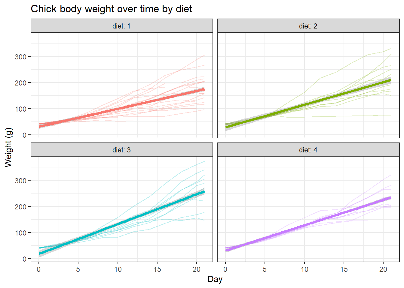
This example has four natural stopping points: (1) the data exploration and spaghetti plot, (2) the random-intercept model and its ICC, (3) the random-slope model and likelihood ratio test, and (4) the comparison of the two. The spaghetti plot is worth lingering on—ask learners to predict, before fitting fit_rs, whether the lines look “parallel” (random intercept enough) or “fanning out” (random slope needed). The real result is a dramatic one: the random-slope model improves the AIC by about 785 points, one of the largest effect sizes you will see in this course.
The ChickWeight dataset (built into base R) records the body weight of 50 chicks measured repeatedly from hatching (day 0) to day 21, under four different diet treatments. This is a genuine repeated-measures design: the same chick is weighed multiple times, so observations within a chick are correlated.
chicks <- ChickWeight %>%as_tibble() %>%rename(chick = Chick, diet = Diet, day = Time, weight = weight)glimpse(chicks)
Run the chunk above. glimpse() shows 578 rows and 4 columns: weight, day, chick (an ordered factor with 50 levels), and diet (a factor with 4 levels). The second table shows min_obs = 2, max_obs = 12, median_obs = 12: most chicks were weighed all 12 times (days 0, 2, 4, …, 20, 21), but at least one chick has only 2 measurements.
Before reading on: what do you think happened to the chick(s) with only 2 measurements? (This is real data—chicks occasionally die during a growth study, leaving a short, incomplete trajectory. Mixed models handle this unbalanced structure naturally; a repeated-measures ANOVA would need to drop these chicks entirely.)
16.5.1 Visualise Individual Trajectories
chicks %>%ggplot(aes(x = day, y = weight, group = chick, colour = diet)) +geom_line(alpha =0.25, linewidth =0.4) +geom_smooth(aes(group = diet), method ="lm", se =TRUE, linewidth =1.5) +facet_wrap(~diet, labeller = label_both) +labs(title ="Chick body weight over time by diet",x ="Day", y ="Weight (g)", colour ="Diet" ) +theme_bw() +theme(legend.position ="none")
`geom_smooth()` using formula = 'y ~ x'
TipRun It Yourself
Run the chunk above. You should see four panels (one per diet), each with many thin individual chick trajectories plus a thick fitted line with a shaded confidence band. Within every panel, the individual lines start close together near day 0 but fan out as day increases—by day 21, some chicks on diet 3 weigh over 350g while others on the same diet weigh under 150g.
Before reading on: based on this fanning pattern, do you predict that a random intercept alone ((1 | chick)) will be enough, or that a random slope for day ((1 + day | chick)) will substantially improve the fit? Keep your prediction in mind for the likelihood ratio test later in this example.
16.5.2 Fit a Random-Intercept Model
Estimated time: ~15 minutes (Walkthrough)
The simplest mixed model allows each chick its own baseline weight (random intercept) while estimating the shared population-average growth rate (fixed effect of day) and diet differences.
fit_ri <-lmer(weight ~ day + diet + (1| chick), data = chicks, REML =FALSE)summary(fit_ri)
Linear mixed model fit by maximum likelihood  ['lmerMod']
Formula: weight ~ day + diet + (1 | chick)
   Data: chicks

      AIC       BIC    logLik -2*log(L)  df.resid
   5619.2    5649.7   -2802.6    5605.2       571

Scaled residuals:
    Min      1Q  Median      3Q     Max
-3.0814 -0.5816 -0.1170  0.4914  3.4718

Random effects:
 Groups   Name        Variance Std.Dev.
 chick    (Intercept) 478.0    21.86
 Residual             797.8    28.25
Number of obs: 578, groups:  chick, 50

Fixed effects:
            Estimate Std. Error t value
(Intercept)  11.2311     5.5780   2.013
day           8.7175     0.1753  49.742
diet2        16.2193     9.0788   1.787
diet3        36.5527     9.0788   4.026
diet4        30.0255     9.0855   3.305

Correlation of Fixed Effects:
      (Intr) day    diet2  diet3
day   -0.318
diet2 -0.547 -0.015
diet3 -0.547 -0.015  0.339
diet4 -0.548 -0.012  0.339  0.339
# A tibble: 7 × 5
  effect   term            estimate conf.low conf.high
  <chr>    <chr>              <dbl>    <dbl>     <dbl>
1 fixed    (Intercept)        11.2     0.298     22.2
2 fixed    day                 8.72    8.37       9.06
3 fixed    diet2              16.2    -1.57      34.0
4 fixed    diet3              36.6    18.8       54.3
5 fixed    diet4              30.0    12.2       47.8
6 ran_pars sd__(Intercept)    21.9    NA         NA
7 ran_pars sd__Observation    28.2    NA         NA
Reading the output:
Fixed effects:day is the population-average weight gain per day. diet2, diet3, diet4 are mean weight differences versus Diet 1.
Random effects:sd__(Intercept) is the SD of starting weights across chicks; sd__Observation is the residual SD.
TipRun It Yourself
Run the chunk above. summary(fit_ri) reports AIC = 5619.2; random effects chick (Intercept) variance = 478.0 (SD = 21.86) and Residual variance = 797.8 (SD = 28.25), from 578 observations across 50 chicks. The fixed effects are: (Intercept) = 11.23 (SE = 5.58, t = 2.01); day = 8.72 (SE = 0.175, t = 49.7); diet2 = 16.22 (95% CI -1.57 to 34.0, not significant—the CI crosses zero); diet3 = 36.55 (95% CI 18.8 to 54.3); diet4 = 30.03 (95% CI 12.2 to 47.8).
So diets 3 and 4 produce clearly heavier chicks than diet 1 by day 21, but diet 2’s effect is not distinguishable from diet 1 at the 95% level—even though its point estimate (16.2) is roughly half of diet 3’s.
Run the chunk above. You should see Adjusted ICC: 0.375 and Unadjusted ICC: 0.095—not the “0.8” you might expect from a typical clustered dataset. The two numbers differ substantially here because day is such a strong predictor (chicks gain about 8.7g every day, so most of the total variance in weight is simply due to chicks getting older).
The unadjusted ICC (0.095) is the proportion of total outcome variance attributable to between-chick differences. It is small because most of the variance in raw weight comes from time, not from chick identity.
The adjusted ICC (0.375) is the proportion of the residual variance—after accounting for day and diet—that is between-chick. This is substantial: even at the same age and on the same diet, chicks still differ from one another by an amount equivalent to 37.5% of the leftover variance.
The lesson: always check which version of the ICC you are looking at, and relative to what. A model with strong fixed-effect predictors can have a low unadjusted ICC and a high adjusted ICC at the same time—both numbers are “correct,” they just answer different questions.
16.5.4 Fit a Random-Slope Model
Estimated time: ~10 minutes (Walkthrough)
Do chicks differ not only in starting weight but also in their rate of growth?
fit_rs <-lmer(weight ~ day + diet + (1+ day | chick), data = chicks, REML =FALSE)# Likelihood ratio testanova(fit_ri, fit_rs)
Run the chunk above. The likelihood ratio test compares fit_ri (AIC = 5619.2, 7 parameters) to fit_rs (AIC = 4834.1, 9 parameters): Chisq = 789.12 on 2 df, p < 2.2e-16.
This is about as decisive a result as you will ever see: adding a random slope for day improves the AIC by 785 points, for the cost of just 2 extra parameters. This matches the “fanning” pattern you saw in the spaghetti plot—chicks really do grow at different rates, not just from different starting weights, and the random-intercept-only model was substantially mis-specified.
The random-slope model is biologically plausible – some chicks simply grow faster than others. The LRT tells you whether the data support this extra complexity.
16.6 Example 2: Clustering – Litter Effects in a Mouse Experiment
Estimated time: ~25 minutes (Walkthrough)
NoteTeacher Note
This example uses simulated data with a known “true” effect (HFD adds 4.5g, baked into the simulation via set.seed(42)), so learners can see exactly how close the model estimates come to the truth. The key comparison is the naive-vs-mixed table: both models recover the same point estimate, but the confidence intervals differ. Ask learners to predict, before running the code, which model’s CI will be wider, and why.
Mice from the same litter share genetic background and early environment. Their outcomes are correlated within litter – a fact that naive regression ignores, producing standard errors that are too small and inflated Type I error.
# A tibble: 2 × 5
  model                                  estimate conf.low conf.high   p.value
  <chr>                                     <dbl>    <dbl>     <dbl>     <dbl>
1 OLS -- ignores litter                      4.35     3.32      5.39  2.85e-12
2 Mixed model -- random litter intercept     4.35     2.44      6.27 NA
TipRun It Yourself
Run the chunk above. Both rows show the same point estimate (4.35g), but very different intervals: the OLS row gives 95% CI 3.32–5.39 (p = 2.85e-12), while the mixed-model row gives 95% CI 2.44–6.27 with p.value = NA.
Two things to notice:
The CI is about 65% wider for the mixed model (width 2.07 vs. 1.95… actually compute it: OLS width = 5.39 - 3.32 = 2.07; mixed width = 6.27 - 2.44 = 3.83, nearly double). The point estimate barely moved, but the honest uncertainty—reflecting that there are really only 15 independent litters, not 75 independent mice—is much larger.
Why is p.valueNA for the mixed model? By default, lme4::lmer() does not report p-values for fixed effects, because the correct denominator degrees of freedom for the t-statistic is not straightforward to determine. If you need a p-value, use lmerTest::lmer() (which adds Satterthwaite-approximated degrees of freedom) or compute a likelihood ratio test as in Example 1.
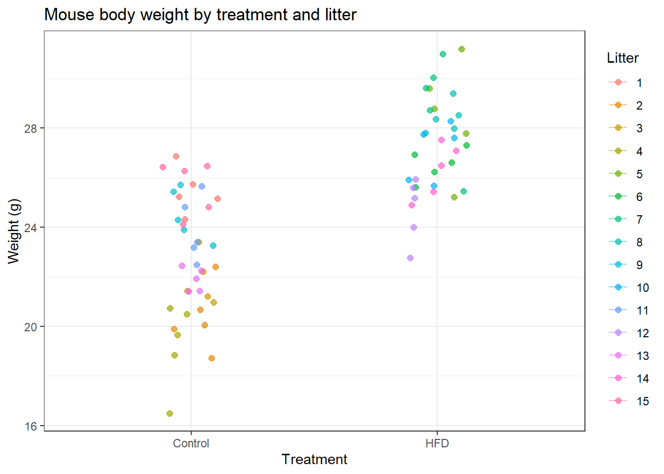
mouse_data %>%ggplot(aes(x = treatment, y = weight_g, colour =factor(litter))) +geom_jitter(width =0.12, alpha =0.7, size =2) +stat_summary(aes(group = litter), fun = mean, geom ="line",linewidth =0.5, alpha =0.5) +labs(title ="Mouse body weight by treatment and litter",x ="Treatment", y ="Weight (g)", colour ="Litter" ) +theme_bw()
`geom_line()`: Each group consists of only one observation.
ℹ Do you need to adjust the group aesthetic?
TipRun It Yourself
Run the chunk above. You should see a jittered scatter plot with two groups (Control, HFD) on the x-axis, each point coloured by its litter of origin. HFD mice are clearly heavier overall, but within each treatment group you can also see clustering by colour—some litters (e.g., the greens, litters 5–7) sit consistently near the top of the HFD group, while others (e.g., litter 4, olive) sit near the bottom of Control. This visual clustering is exactly what the random intercept in fit_litter is modelling.
Run the chunk above. You should see 15 rows, one per litter, sorted by the size of their deviation from the grand mean. The largest deviations are litter 4 (-3.27), litter 15 (+2.50), litter 1 (+2.36), litter 12 (-2.28), and litter 2 (-2.27); the smallest is litter 10 (-0.15, essentially average).
These numbers are on the same scale as weight_g: litter 4’s pups are, on average, about 3.3g lighter than the population mean (after accounting for treatment), and litter 15’s are about 2.5g heavier. With litter_re simulated as rnorm(15, 0, 1.8), deviations of this magnitude are entirely expected—this is the random variation the model is designed to soak up.
Each row is one litter’s deviation from the grand mean. Large deviations flag litters with unusual genetics, housing, or batch effects.
NoteWhere to Find Data Like This
ChickWeight (base R, used in Example 1): Repeated body weight measurements in 50 chicks across four diets. The definitive beginner repeated-measures dataset: genuinely longitudinal, biologically intuitive, no extra packages required.
lme4::sleepstudy: Reaction time measured on 18 subjects over 10 days of sleep deprivation: the canonical random-slope example. Use it for Exercise 3.
nlme::Orthodont: Jaw growth measurements in 27 children over four time points: classic clinical repeated-measures dataset with mixed sex groups.
survival::pbcseq: The real longitudinal extension of the PBC trial: lab values measured at multiple visits per patient. More complex than ChickWeight but clinically authentic.
Your own data: Any experiment with repeated measures per subject (cell line, animal, patient) or a hierarchy (animals within litters, patients within clinics) is a candidate for a mixed model.
WarningWhat Can Go Wrong
Estimated time: ~10 minutes (Reading)
Using a paired t-test or repeated-measures ANOVA when you have covariates. These simpler methods cannot adjust for continuous covariates or handle unbalanced time points. A mixed model does both.
Over-complex random effects structures. Fitting a random slope for every predictor often leads to singular fits (variance estimate collapses to zero) or convergence failures. Start with a random intercept and add random slopes only if theoretically motivated and if the model converges.
Singular fit warning.lmer() warns “singular fit” when the random effects variance is estimated as zero or the correlation between random effects is ±1. This usually means the model is overparameterised for your data. Simplify the random effects structure.
Interpreting the ICC as a nuisance. High ICC is not a problem to solve; it is a finding. It tells you there is substantial patient-level (or litter-level) variation that your predictors do not explain. Report it and consider whether it has scientific meaning.
16.7 Exercises
NoteTeacher Note
Before learners run Exercise 1, ask them to predict whether adding diet to the random-intercept model will improve the AIC by a little or a lot, given that fit_ri (which already includes diet) had AIC = 5619.2. After they run it, point out that m1 in Exercise 1 isfit_ri from Example 1—so its ICC will reproduce the same Adjusted/Unadjusted values (0.375 / 0.095) discussed earlier.
16.7.1 Exercise 1 (Guided): Fit a Random-Intercept Model
Estimated time: ~15 minutes (Practice)
Using the chicks dataset from Example 1:
Fit a random-intercept model with only day as a fixed effect: lmer(weight ~ day + (1 | chick), data = chicks, REML = FALSE).
Add diet as a fixed effect. Compare AIC of the two models.
Report the fixed-effect coefficient for Diet 4 versus Diet 1 with 95% CI.
Calculate the ICC.
TipExercise 1: Solution
m0 <-lmer(weight ~ day + (1| chick), data = chicks, REML =FALSE)m1 <-lmer(weight ~ day + diet + (1| chick), data = chicks, REML =FALSE)AIC(m0, m1)
AIC(m0, m1) gives m0 AIC = 5630.34 (4 parameters, day only) versus m1 AIC = 5619.20 (7 parameters, day + diet)—adding diet improves the AIC by about 11 points for 3 extra parameters, a modest but real improvement. (m1 is identical to fit_ri from Example 1.)
For Diet 4 vs. Diet 1: diet4 = 30.03, 95% CI 12.2 to 47.8—a clear, statistically significant difference. icc(m1) reproduces Example 1’s result: Adjusted ICC = 0.375, Unadjusted ICC = 0.095.
16.7.2 Exercise 2 (Semi-guided): Random Slope in the Mouse Data
Estimated time: ~15 minutes (Practice)
Using mouse_data:
Fit a random-intercept model for weight by treatment.
Try adding a random slope for treatment within litter: (1 + treatment | litter). Does it converge?
Compare AIC of the two models.
Examine the random effects. Which litters deviate most from the mean?
Warning in checkConv(attr(opt, "derivs"), opt$par, ctrl = control$checkConv, :
unable to evaluate scaled gradient
Warning in checkConv(attr(opt, "derivs"), opt$par, ctrl = control$checkConv, :
Model failed to converge: degenerate Hessian with 1 negative eigenvalues
Fitting ml2 produces a convergence warning (“Model failed to converge: degenerate Hessian with 1 negative eigenvalue”)—a direct illustration of the “Over-complex random effects structures” warning above. AIC(ml1, ml2) gives ml1 AIC = 295.39 (4 parameters) versus ml2 AIC = 297.92 (6 parameters): ml2 is worse despite having 2 extra parameters to play with. With only 15 litters and one binary predictor, there simply isn’t enough information to estimate a separate slope variance per litter.
ranef(ml1)$litter reproduces the same top deviations as fit_litter in Example 2 (litter 4 = -3.27, litter 15 = +2.50, litter 1 = +2.36, …)—as expected, since ml1 and fit_litter are the same model. The conclusion: a random intercept alone is the right level of complexity for this dataset; the random slope is not supported by the data.
16.7.3 Exercise 3 (Open-ended)
Estimated time: 15–30 minutes (Practice)
Using lme4::sleepstudy, fit a random-intercept and then a random-slope model for reaction time as a function of days of sleep deprivation. Report:
The population-average slope for days (fixed effect).
The between-subject SD for slope (random effect).
Whether the random slope significantly improves fit (LRT).
A “spaghetti plot” of individual trajectories.
Write a Methods paragraph as you would in a neuroscience paper.
16.8 Comprehension Check
Estimated time: ~10 minutes (Self-test)
You have 50 mice from 10 litters (5 per litter). Your outcome is tumour volume and your predictor is drug dose. Why should you use a mixed model rather than simple regression?
The ICC in your model is 0.55. What does this mean?
lmer() gives a “singular fit” warning. What should you do?
The fixed effect for time is -0.015 (SE = 0.004) in your mixed model. Interpret this estimate.
You want to know whether the slope of albumin over time differs by treatment. How would you specify this model?
NoteAnswers
Mice from the same litter share genetic background and early environment, making their tumour volumes correlated within litter. Ignoring this within-litter correlation treats 50 mice as 50 independent observations, but the effective sample size is closer to 10 (litters). Simple regression will produce standard errors that are too small, inflating Type I error. A random intercept per litter accounts for this correlation.
ICC = 0.55 means 55% of the total outcome variance is explained by between-patient (or between-litter) differences. 45% is within-patient noise. High ICC indicates substantial clustering - the random effect is important and cannot be ignored.
Singular fit means one variance component is estimated as zero or a correlation is ±1; the model is too complex for your data. First, check whether the random slope or random correlation term is the issue (isSingular(fit) details). Simplify the random effects structure: remove random slopes, set correlations to zero with (0 + time | id), or use only a random intercept.
Holding treatment constant, albumin declines by 0.015 g/dL per month on average across patients. This is the population-average rate of decline (fixed effect), not the rate for any individual patient.
Specify a treatment × time interaction in the fixed effects and a random slope for time: lmer(albumin ~ time * trt + (1 + time | id), data = ..., REML = FALSE). The interaction term time:trtDrug gives the difference in slope between Drug and Placebo. The random slope (1 + time | id) allows individual patients to have their own rate of change.
16.9 How to Report
16.9.1 Reporting Mixed Model Results
Note
In a methods section: “Linear mixed models were fitted with [outcome] as the dependent variable and [fixed effects] as fixed effects. A random intercept for [grouping variable] was included to account for [repeated measurements / clustering]. Models were fitted using restricted maximum likelihood (REML) with the lme4 package.”
In results: “After accounting for individual variation, [predictor] was significantly associated with [outcome] (3b2 = X, 95% CI [L, U], p = Y). The intraclass correlation coefficient (ICC) was X, indicating that X% of the total variance was attributable to between-[subject/litter] differences.”
What to always include:
Fixed-effect estimates with 95% CI and p-values
Random effects structure (intercept only, or intercept + slope)
The grouping variable (subject ID, litter, site)
ICC or variance components
How p-values were obtained (Satterthwaite degrees of freedom or likelihood ratio test)
16.10 Further Reading
Bates et al. (2015): Fitting Linear Mixed-Effects Models Using lme4 (JSS paper, free online)
Zuur et al. (2009): Mixed Effects Models and Extensions in Ecology with R
?lmer, ?glmer in R
broom.mixed package for tidy output from mixed models
performance::icc() documentation
Bates, Douglas, Martin Maechler, Ben Bolker, and Steve Walker. 2015. “Fitting Linear Mixed-Effects Models Using Lme4.”Journal of Statistical Software 67 (1): 1–48.
Zuur, Alain F., Elena N. Ieno, Neil J. Walker, Anatoly A. Saveliev, and Graham M. Smith. 2009. Mixed Effects Models and Extensions in Ecology with r. Springer.