15  Missing Data and Imputation

NoteSession at a Glance

Total core time: ~160 minutes (about 2.5–3 hours). If you need to split this across sessions, a natural break point is after the complete-case analysis (end of “Complete-Case Analysis (Baseline)”)—cover the multiple-imputation comparison and Example 2 in a second sitting. Exercise 3 is open-ended and its time will vary with your own data.

Section	Time	Type
The Key Idea: Three Mechanisms	~10 min	Concept
Background: Why Missing Data Matter	~15 min	Concept
Example 1: Clinical Data (PBC)	~50 min	Walkthrough
Example 2: Penguins Data	~15 min	Walkthrough
What Can Go Wrong	~10 min	Reading
Exercise 1 (Guided)	~15 min	Practice
Exercise 2 (Semi-guided)	~20 min	Practice
Exercise 3 (Open-ended)	15–30 min	Practice
Comprehension Check	~10 min	Self-test

If you are short on time, the single most important result in this session is the compare table near the end of Example 1: it shows directly how much complete-case analysis can diverge from a properly imputed analysis.

TipHow to Use the Code in This Session

Every code chunk below is written so you can copy it into your R console (or an R script) and run it yourself, in the order shown. Where you see a “Run It Yourself” box, stop and run the code above it before reading the explanation that follows.

15.1 When Do You Use This?

Tip

Your dataset has missing values. Simply dropping incomplete cases loses statistical power, and if data are not missing at random, dropping them biases your estimates in ways that are difficult to detect. Missing data methods let you use all available information and make your assumptions about missingness explicit. For example: if sicker patients are more likely to have missing lab values, a complete-case analysis systematically excludes the most severely ill and distorts every downstream estimate.

NoteTeacher Note

Before running anything, ask learners to predict: in the PBC dataset, which lab values do they expect to have the most missingness, and why? (Hint: this is a study that recruited patients over many years, and some tests were added partway through the study.) The real answer—trig and chol are each missing for about a third of patients—often surprises learners who expect missingness to be rare. This sets up the “Exploring Missingness” section nicely.

15.2 Learning Objectives

After completing this session you will be able to:

• Classify missing data as MCAR, MAR, or MNAR and explain why the distinction matters
• Explore missingness patterns and assess whether missingness is related to other variables
• Implement complete-case analysis and explain when it is valid
• Perform multiple imputation with mice and combine results using Rubin’s rules
• Report imputed analyses correctly in a manuscript

15.3 The Key Idea: Three Mechanisms, Three Consequences

Estimated time: ~10 minutes (Concept)

The most important concept in missing data is why values are missing. The answer determines what you can validly do about it.

Think of it this way: imagine you are measuring blood pressure. Some readings are missing because the machine broke randomly: that is truly random, unrelated to anything else. Some are missing because elderly patients were too tired to attend follow-up (missingness depends on their age, which you can observe). And some are missing because patients with dangerously high pressure were admitted to hospital before the reading (missingness depends on the very thing you are trying to measure, which you cannot observe).

Those three scenarios have completely different consequences for your analysis.

15.4 Background: Why Missing Data Matter

Estimated time: ~15 minutes (Concept)

15.4.1 Three Mechanisms

Mechanism	Definition	Implication
MCAR: Missing Completely At Random	Probability of missing is unrelated to any variable	Complete-case analysis is unbiased
MAR: Missing At Random	Probability of missing depends on observed variables, not on the missing value itself	Multiple imputation is valid; complete-case is biased
MNAR: Missing Not At Random	Probability of missing depends on the unobserved missing value itself	Neither complete-case nor simple imputation is valid; sensitivity analysis required

Example: Patients with high bilirubin are less likely to have platelet counts recorded (perhaps because they were too ill for the test). Missingness depends on observed bilirubin (MAR). Imputation conditioned on bilirubin will recover unbiased estimates.

15.4.2 Why Not Just Drop Missing Rows?

Complete-case analysis:

• Reduces sample size and loses statistical power
• Is biased under MAR or MNAR
• Implicitly assumes MCAR: an assumption you should test, not ignore

15.4.3 Multiple Imputation Overview

Multiple imputation (MI) replaces each missing value with \(m\) plausible draws from the conditional distribution of the missing variable given the observed data. This produces \(m\) complete datasets. Each is analysed separately and results are combined using Rubin’s rules, which pool point estimates and propagate the extra uncertainty due to imputation into the standard errors.

15.5 Example 1: Clinical Data (PBC)

Estimated time: ~50 minutes (Walkthrough)

NoteTeacher Note

This example has five natural stopping points: (1) the missingness table, (2) the bilirubin-by-missingness plot, (3) the complete-case fit, (4) the mice trace plots and pooled fit, and (5) the side-by-side comparison table. The comparison table is the payoff for the whole example—make sure learners reach it, even if you need to move quickly through earlier sections. Little’s MCAR test requires the naniar package, which is not installed in every environment; if it is not available, skip straight from the exploratory plot to the complete-case analysis.

15.5.1 Exploring Missingness

Estimated time: ~15 minutes (Walkthrough)

pbc <- survival::pbc %>%
  as_tibble() %>%
  clean_names()

pbc %>%
  summarise(across(everything(), \(x) mean(is.na(x)))) %>%
  pivot_longer(everything(), names_to = "variable", values_to = "prop_missing") %>%
  filter(prop_missing > 0) %>%
  arrange(desc(prop_missing))

# A tibble: 12 × 2
   variable prop_missing
   <chr>           <dbl>
 1 trig          0.325  
 2 chol          0.321  
 3 copper        0.258  
 4 trt           0.254  
 5 ascites       0.254  
 6 hepato        0.254  
 7 spiders       0.254  
 8 alk_phos      0.254  
 9 ast           0.254  
10 platelet      0.0263 
11 stage         0.0144 
12 protime       0.00478

TipRun It Yourself

Run the chunk above. You should see a 12-row table sorted by prop_missing, with trig (0.325) and chol (0.321) at the top—about a third of patients are missing these. copper, trt, ascites, hepato, spiders, alk_phos, and ast are all missing for about a quarter (0.254) of patients, platelet for 2.6%, stage for 1.4%, and protime for less than 0.5%.

Before reading on: does a third of patients missing trig and chol surprise you? What might explain such a high rate for these two variables specifically, when albumin and bili have no missing values at all?

vis_miss(pbc %>% select(albumin, bili, platelet, protime, chol, trig, copper))

NoteTeacher Note

The vis_miss() plot above requires the naniar package. If naniar is not installed, this chunk produces no output at all—install it with install.packages("naniar") to see a heatmap of missingness across every variable and observation at once. The histogram in the next chunk (miss-gg) works without any extra packages and tells a similar story for one variable at a time.

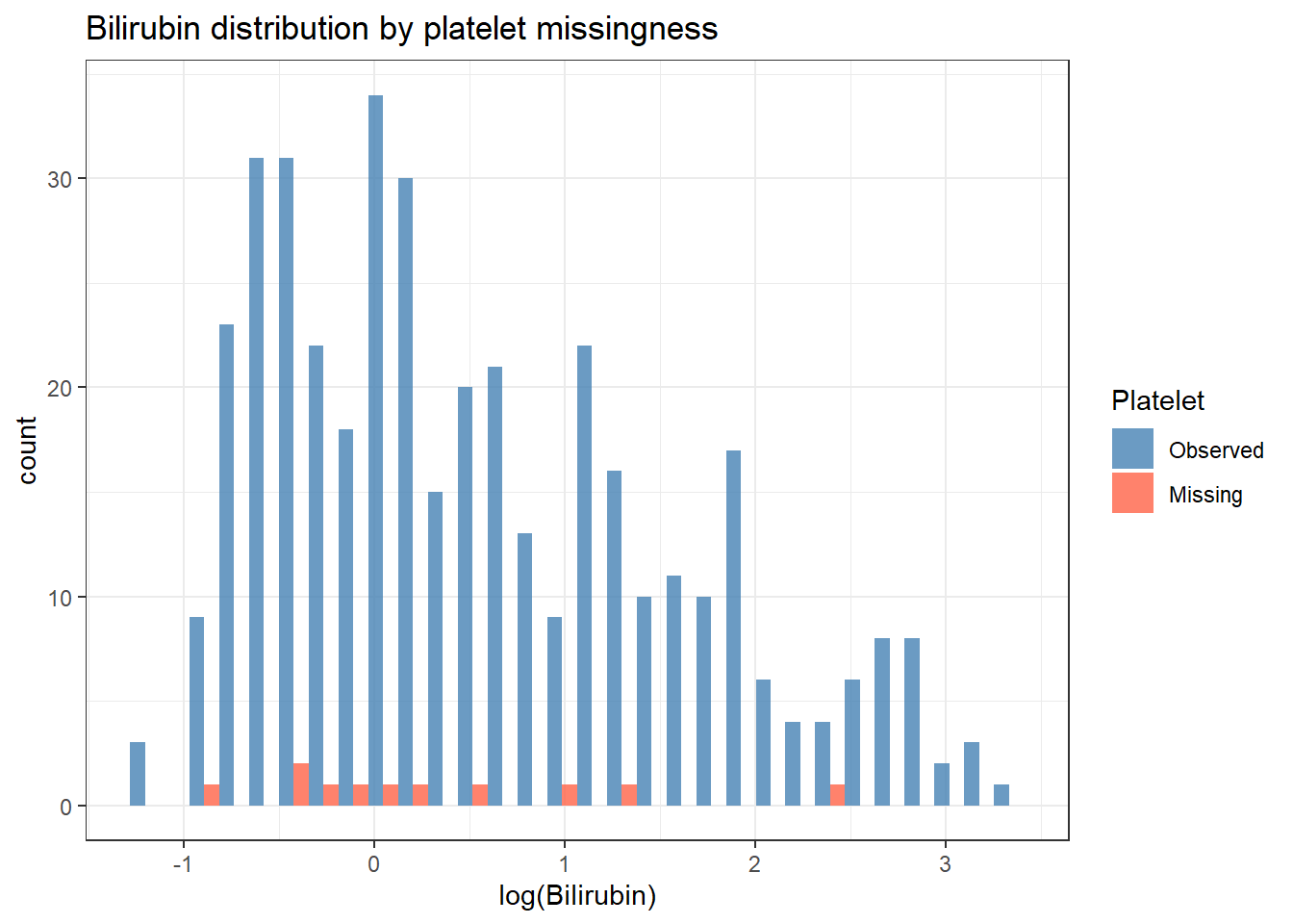
pbc %>%
  mutate(platelet_missing = is.na(platelet)) %>%
  ggplot(aes(x = log(bili), fill = platelet_missing)) +
  geom_histogram(position = "dodge", bins = 30, alpha = 0.8) +
  scale_fill_manual(values = c("steelblue", "tomato"),
                    labels = c("Observed", "Missing")) +
  labs(title = "Bilirubin distribution by platelet missingness",
       x = "log(Bilirubin)", fill = "Platelet") +
  theme_bw()

TipRun It Yourself

Run the chunk above. You should see a histogram of log(bili) with two overlapping bars at each bin: blue for patients with an observed platelet count, and orange/red for patients with a missing platelet count. The red bars appear scattered across most of the range of log(bili), from about -1 to 2.5, rather than clustering at one end.

This is a useful preview: if missingness were strongly tied to bilirubin, you’d expect the red bars to cluster at high (or low) values of log(bili). They don’t obviously do so here—keep this in mind for Exercise 1, which tests this relationship formally.

If the distributions differ, missingness is related to bilirubin, consistent with MAR rather than MCAR.

15.5.2 Little’s MCAR Test

Estimated time: ~5 minutes (Reading)

mcar_test(pbc %>% select(albumin, bili, platelet, protime, chol))

A significant p-value (p < 0.05) means the data are not MCAR. In that case, complete-case analysis is biased and multiple imputation is necessary.

NoteTeacher Note

mcar_test() is part of the naniar package and, like vis_miss() above, produces no output if naniar is not installed. Where it is available, it returns a chi-squared statistic and p-value: a significant result (p < 0.05) is evidence against MCAR. Don’t over-interpret a non-significant result as proof of MCAR, though—the test has limited power and cannot detect MNAR at all. The complete-case vs. multiple-imputation comparison later in this example is a more practical check: if the two sets of estimates differ substantially, that is direct evidence that complete-case analysis is doing something different from MI.

15.5.3 Complete-Case Analysis (Baseline)

Estimated time: ~10 minutes (Walkthrough)

pbc_cc <- pbc %>%
  filter(!is.na(albumin), !is.na(bili), !is.na(platelet), !is.na(protime), !is.na(stage)) %>%
  mutate(
    log_bili = log(bili),
    stage    = factor(stage, levels = 1:4, labels = paste("Stage", 1:4))
  )

cat("Complete cases:", nrow(pbc_cc), "of", nrow(pbc), "\n")

Complete cases: 399 of 418 

fit_cc <- lm(albumin ~ log_bili + platelet + stage, data = pbc_cc)
broom::tidy(fit_cc, conf.int = TRUE) %>%
  select(term, estimate, conf.low, conf.high, p.value)

# A tibble: 6 × 5
  term          estimate   conf.low conf.high   p.value
  <chr>            <dbl>      <dbl>     <dbl>     <dbl>
1 (Intercept)   3.61      3.41       3.82     4.81e-120
2 log_bili     -0.106    -0.144     -0.0670   1.30e-  7
3 platelet      0.000385 -0.0000237  0.000793 6.48e-  2
4 stageStage 2 -0.0903   -0.280      0.0998   3.51e-  1
5 stageStage 3 -0.0766   -0.260      0.107    4.12e-  1
6 stageStage 4 -0.300    -0.489     -0.112    1.88e-  3

TipRun It Yourself

Run the chunk above. You should see:

• Complete cases: 399 of 418—19 patients (4.5%) are dropped entirely, even though most of them have only one or two missing values.
• fit_cc coefficients: log_bili = -0.106 (95% CI -0.144 to -0.067, p < 0.001); platelet = 0.000385 (95% CI -0.0000237 to 0.000793, p = 0.065, not significant); stageStage 4 = -0.300 (95% CI -0.489 to -0.112, p = 0.002); stageStage 2 and stageStage 3 are both non-significant (p = 0.351 and p = 0.412).

So in the complete-case analysis, only log_bili and stage 4 are clearly associated with albumin. Keep these numbers in mind—you’ll compare them directly to the multiply-imputed estimates shortly.

15.5.4 Multiple Imputation with mice

Estimated time: ~15 minutes (Walkthrough)

pbc_imp <- pbc %>%
  select(albumin, bili, platelet, protime, chol, trig, copper, stage, age, sex) %>%
  mutate(
    log_bili  = log(bili),
    stage     = factor(stage, levels = 1:4),
    sex       = factor(sex)
  ) %>%
  select(-bili)

set.seed(2024)
imp <- mice(pbc_imp, m = 10, method = "pmm", printFlag = FALSE)

plot(imp, c("platelet", "chol"), layout = c(2, 2))

TipRun It Yourself

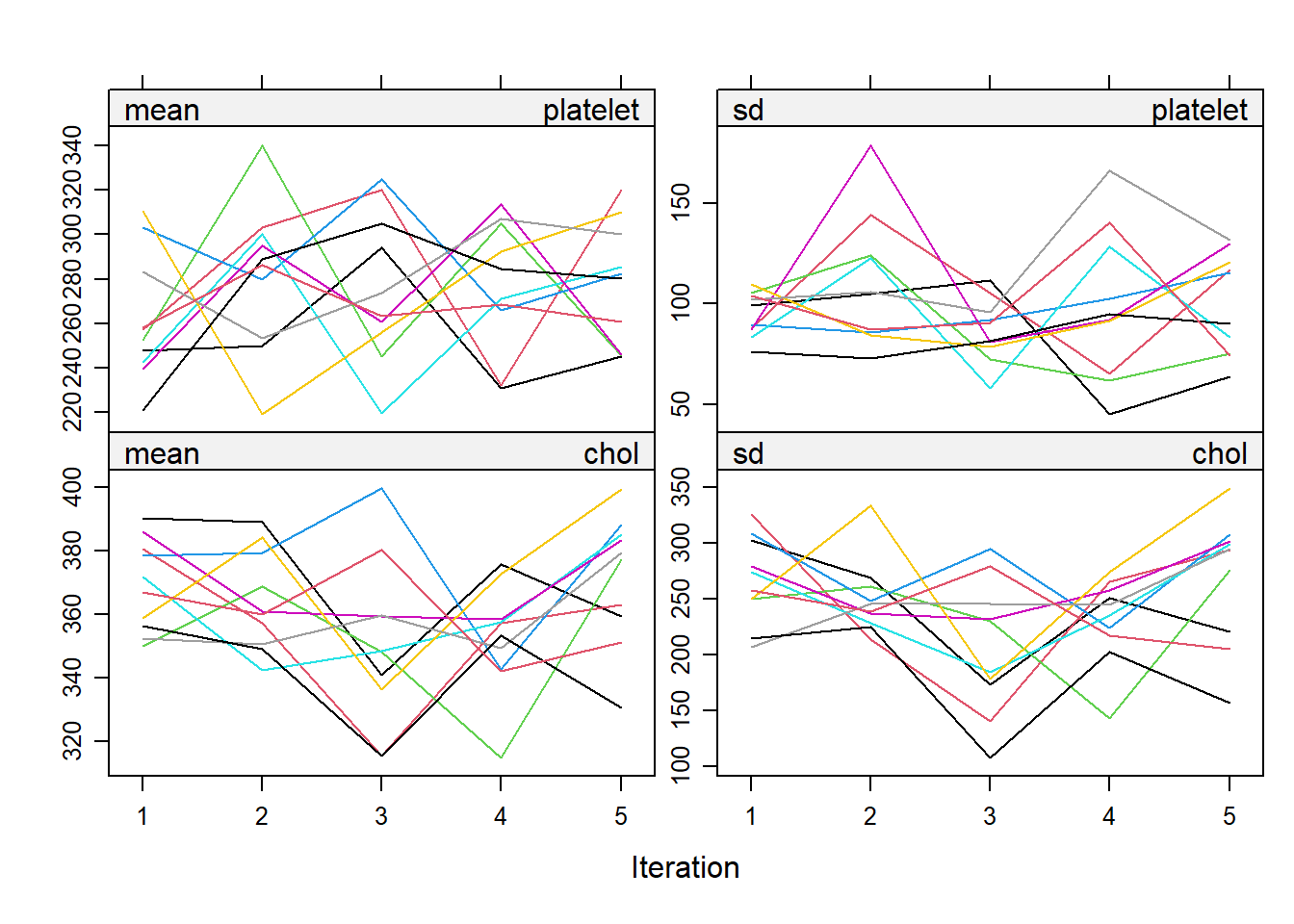
Run the chunk above. You should see a 2x2 grid of trace plots: mean and standard deviation of the imputed values for platelet (top row) and chol (bottom row), across 5 iterations, with one line per imputed dataset (m = 10 lines).

Good convergence looks like the lines criss-crossing back and forth without any overall upward or downward drift—a “fat hairball” rather than lines that diverge or trend in one direction. The plots above show exactly this: the lines for both variables wander up and down across iterations but show no systematic trend, which is what you want to see.

The trace plots should mix well (lines criss-crossing rather than staying in one area): this indicates the imputation algorithm has converged.

fit_mi <- with(imp, lm(albumin ~ log_bili + platelet + stage))
pooled  <- pool(fit_mi)
summary(pooled, conf.int = TRUE) %>%
  select(term, estimate, `2.5 %`, `97.5 %`, p.value)

         term      estimate         2.5 %        97.5 %       p.value
1 (Intercept)  3.5924121923  3.389161e+00  3.7956632913 2.045943e-118
2    log_bili -0.1113111172 -1.494265e-01 -0.0731957098  1.837281e-08
3    platelet  0.0003379551 -5.861619e-05  0.0007345263  9.463304e-02
4      stage2 -0.0553859879 -2.413508e-01  0.1305787874  5.584418e-01
5      stage3 -0.0396703823 -2.200122e-01  0.1406714038  6.655526e-01
6      stage4 -0.2603963469 -4.455976e-01 -0.0751950927  5.983364e-03

TipRun It Yourself

Run the chunk above. The pooled multiple-imputation estimates are: log_bili = -0.111 (95% CI -0.149 to -0.073, p < 0.001); platelet = 0.000338 (95% CI -0.0000586 to 0.000735, p = 0.095, not significant); stage2 = -0.055 (p = 0.558), stage3 = -0.040 (p = 0.666), stage4 = -0.260 (95% CI -0.446 to -0.075, p = 0.006).

Compare these to the complete-case numbers from the previous section. The conclusions are broadly similar—log_bili and stage 4 remain significant, platelet and the lower stage categories remain non-significant—but every estimate has shifted slightly, and (as you’ll see in the comparison table next) the standard errors have changed too.

15.5.5 Comparing Complete-Case and Imputed Estimates

Estimated time: ~5 minutes (Walkthrough)

cc_results <- broom::tidy(fit_cc, conf.int = TRUE) %>%
  select(term, estimate, conf.low, conf.high, p.value) %>%
  mutate(method = "Complete-case")

mi_results <- summary(pooled, conf.int = TRUE) %>%
  as_tibble() %>%
  select(term, estimate, conf.low = `2.5 %`, conf.high = `97.5 %`, p.value) %>%
  mutate(method = "Multiple imputation")

bind_rows(cc_results, mi_results) %>%
  filter(term %in% c("log_bili", "platelet",
                     "stageStage 2", "stageStage 3", "stageStage 4")) %>%
  select(method, term, estimate, conf.low, conf.high, p.value) %>%
  arrange(term, method)

# A tibble: 7 × 6
  method              term          estimate   conf.low conf.high      p.value
  <chr>               <chr>            <dbl>      <dbl>     <dbl>        <dbl>
1 Complete-case       log_bili     -0.106    -0.144     -0.0670   0.000000130 
2 Multiple imputation log_bili     -0.111    -0.149     -0.0732   0.0000000184
3 Complete-case       platelet      0.000385 -0.0000237  0.000793 0.0648      
4 Multiple imputation platelet      0.000338 -0.0000586  0.000735 0.0946      
5 Complete-case       stageStage 2 -0.0903   -0.280      0.0998   0.351       
6 Complete-case       stageStage 3 -0.0766   -0.260      0.107    0.412       
7 Complete-case       stageStage 4 -0.300    -0.489     -0.112    0.00188     

TipRun It Yourself

Run the chunk above. You should see a 7-row table:

method	term	estimate	conf.low	conf.high	p.value
Complete-case	log_bili	-0.106	-0.144	-0.0670	1.3e-7
Multiple imputation	log_bili	-0.111	-0.149	-0.0732	1.8e-8
Complete-case	platelet	0.000385	-0.0000237	0.000793	0.065
Multiple imputation	platelet	0.000338	-0.0000586	0.000735	0.095
Complete-case	stageStage 2	-0.0903	-0.280	0.0998	0.351
Complete-case	stageStage 3	-0.0766	-0.260	0.107	0.412
Complete-case	stageStage 4	-0.300	-0.489	-0.112	0.002

Spot the gotcha: there are no “Multiple imputation” rows for stage. Look closely at the filter() step: it keeps terms named "stageStage 2", "stageStage 3", "stageStage 4"—the names produced by fit_cc, where stage was coded as a labelled factor ("Stage 1", …, "Stage 4"). But in pbc_imp, stage was coded as a plain numeric factor (factor(stage, levels = 1:4)), so fit_mi’s terms are named "stage2", "stage3", "stage4"—and these don’t match the filter, so they are silently dropped.

This is a realistic bug: the code runs without error and produces a plausible-looking table, but it is quietly incomplete. From the mice-analyse Run It Yourself box above, you already have the missing numbers: stage2 = -0.055, stage3 = -0.040, stage4 = -0.260 for multiple imputation, versus -0.090, -0.077, -0.300 for complete-case. The biggest gap is stage 4: complete-case overstates the effect (-0.300 vs -0.260)—exactly the kind of bias multiple imputation is meant to correct.

If the estimates differ substantially, the missing data were not MCAR and complete-case analysis was biased.

15.6 Example 2: Penguins Data

Estimated time: ~15 minutes (Walkthrough)

NoteTeacher Note

This example deliberately uses a dataset with very little missingness (palmerpenguins), to show that the MI workflow is the same regardless of how much data is missing—only the consequences differ. Ask learners to predict, before running the code: with only 2 missing values per numeric variable (out of 344 penguins), would they expect the multiply-imputed estimates to differ much from a complete-case analysis here? (They shouldn’t—and that is the point: MI is “do no harm” when missingness is minimal, but essential when it is not, as in the PBC example.)

penguins %>%
  summarise(across(everything(), \(x) sum(is.na(x)))) %>%
  pivot_longer(everything()) %>%
  filter(value > 0)

# A tibble: 5 × 2
  name              value
  <chr>             <int>
1 bill_length_mm        2
2 bill_depth_mm         2
3 flipper_length_mm     2
4 body_mass_g           2
5 sex                  11

TipRun It Yourself

Run the chunk above. You should see a 5-row table: bill_length_mm, bill_depth_mm, flipper_length_mm, and body_mass_g are each missing for 2 penguins (out of 344), and sex is missing for 11. This is a tiny fraction of the data—well under 1% for the numeric variables.

peng_imp <- penguins %>%
  select(body_mass_g, flipper_length_mm, bill_length_mm, bill_depth_mm, species, sex) %>%
  mutate(species = factor(species), sex = factor(sex))

set.seed(2024)
imp_peng <- mice(peng_imp, m = 5, method = "pmm", printFlag = FALSE)

fit_peng <- with(imp_peng, lm(body_mass_g ~ flipper_length_mm + species))
summary(pool(fit_peng), conf.int = TRUE)

               term    estimate  std.error statistic       df      p.value
1       (Intercept) -4015.67592 581.583736 -6.904725 337.7001 2.503282e-11
2 flipper_length_mm    40.62395   3.057504 13.286636 337.7264 1.070355e-32
3  speciesChinstrap  -206.36073  57.561756 -3.585032 337.7124 3.867145e-04
4     speciesGentoo   268.25506  94.906156  2.826530 337.8972 4.985667e-03
        2.5 %      97.5 %    conf.low   conf.high
1 -5159.65904 -2871.69281 -5159.65904 -2871.69281
2    34.60980    46.63810    34.60980    46.63810
3  -319.58547   -93.13598  -319.58547   -93.13598
4    81.57376   454.93637    81.57376   454.93637

TipRun It Yourself

Run the chunk above. The pooled estimates are: (Intercept) = -4015.7 (95% CI -5159.7 to -2871.7); flipper_length_mm = 40.6 (95% CI 34.6 to 46.6, p < 0.001); speciesChinstrap = -206.4 (95% CI -319.6 to -93.1, p < 0.001); speciesGentoo = 268.3 (95% CI 81.6 to 454.9, p = 0.005).

If you re-ran this with na.omit() and a plain lm() instead of mice, you would find the coefficients are nearly identical—because with only 2 missing values per variable, there is very little for imputation to “do.” This confirms the prediction from the Teacher Note above: MI matters most when missingness is substantial, as in the PBC example, not when it is minimal.

NoteWhere to Find Data Like This

survival::pbc: Real-world clinical data with informative missingness in laboratory values, a classic MI teaching example.

palmerpenguins: Minimal missingness; useful to practice the workflow without bias concerns.

NHANES (via the NHANES or nhanesA packages): Large survey with complex, realistic missingness patterns across demographic and clinical variables.

WarningWhat Can Go Wrong

Estimated time: ~10 minutes (Reading)

Imputing the outcome. Never include the outcome variable as a predictor in the imputation model if missingness in the outcome is not informative. Report the proportion of missing outcomes and conduct a sensitivity analysis.

Too few imputed datasets. The rule of thumb is m ≥ the percentage of missing data (e.g., 20% missing → m ≥ 20). Five imputations is typically insufficient when missingness is substantial.

Using complete-case AIC to select variables before imputing. Model selection should be done within the multiply-imputed framework, not on complete cases only. Selecting variables on complete cases and then imputing introduces bias.

MNAR without sensitivity analysis. If you have reason to believe data are MNAR (e.g., lab values missing because the patient refused due to anxiety about results), standard MI is not sufficient. Perform a sensitivity analysis under plausible MNAR scenarios using mice with a delta adjustment.

15.7 Exercises

NoteTeacher Note

Before learners run Exercise 1, ask them to predict: based on the miss-gg plot earlier (which showed missing platelet values scattered across the bilirubin range), do they expect a logistic regression of platelet-missingness on log(bili) to be statistically significant? After they run it, discuss why a non-significant result here does not prove the data are MCAR overall—it only tells you that this one variable does not explain platelet missingness; other variables (e.g., trt, calendar time) might still matter.

15.7.1 Exercise 1 (Guided): Explore PBC Missingness

Estimated time: ~15 minutes (Practice)

1. Count the proportion of missing values for each variable in survival::pbc.
2. Visualise the missingness pattern for platelet, chol, trig, and copper.
3. Test whether missingness in platelet is associated with bili (logistic regression). What does a significant result tell you?

TipExercise 1: Solution

pbc %>%
  summarise(across(everything(), \(x) mean(is.na(x)))) %>%
  pivot_longer(everything()) %>%
  filter(value > 0) %>%
  arrange(desc(value))

# A tibble: 12 × 2
   name       value
   <chr>      <dbl>
 1 trig     0.325  
 2 chol     0.321  
 3 copper   0.258  
 4 trt      0.254  
 5 ascites  0.254  
 6 hepato   0.254  
 7 spiders  0.254  
 8 alk_phos 0.254  
 9 ast      0.254  
10 platelet 0.0263 
11 stage    0.0144 
12 protime  0.00478

pbc_test <- pbc %>% mutate(platelet_miss = as.integer(is.na(platelet)))
glm(platelet_miss ~ log(bili), data = pbc_test, family = binomial) %>%
  broom::tidy(conf.int = TRUE, exponentiate = TRUE)

# A tibble: 2 × 7
  term        estimate std.error statistic  p.value conf.low conf.high
  <chr>          <dbl>     <dbl>     <dbl>    <dbl>    <dbl>     <dbl>
1 (Intercept)   0.0306     0.324   -10.8   4.75e-27   0.0150    0.0543
2 log(bili)     0.758      0.332    -0.836 4.03e- 1   0.369     1.38  

The missingness table reproduces the 12-row result from “Exploring Missingness” above (trig 0.325, chol 0.321, …, protime 0.00478).

For the logistic regression, log(bili) has OR ≈ 0.758 (95% CI 0.369–1.38, p ≈ 0.40)—not statistically significant. So in this univariable test, missingness in platelet is not detectably associated with bilirubin, consistent with the scattered pattern you saw in the miss-gg plot. This does not prove the data are MCAR (the test has limited power, and other variables could still be related to platelet missingness), but it is at least reassuring: the variable most central to this session’s analyses (log_bili) does not appear to drive platelet missingness on its own.

15.7.2 Exercise 2 (Semi-guided): Multiple Imputation of PBC

Estimated time: ~20 minutes (Practice)

1. Select variables: albumin, log_bili, platelet, chol, stage.
2. Create 20 imputed datasets using mice with method = "pmm".
3. Fit lm(albumin ~ log_bili + platelet + stage) in each and pool.
4. Compare pooled SEs to the complete-case SEs. Which are larger, and why?

TipExercise 2: Solution

pbc_ex <- pbc %>%
  mutate(log_bili = log(bili), stage = factor(stage)) %>%
  select(albumin, log_bili, platelet, chol, stage)

set.seed(42)
imp_ex <- mice(pbc_ex, m = 20, method = "pmm", printFlag = FALSE)

fit_ex2 <- with(imp_ex, lm(albumin ~ log_bili + platelet + stage))
summary(pool(fit_ex2), conf.int = TRUE)

         term      estimate    std.error  statistic       df       p.value
1 (Intercept)  3.6085482116 0.1026285377 35.1612553 402.6201 8.476188e-125
2    log_bili -0.1116984109 0.0193911974 -5.7602637 409.4122  1.651924e-08
3    platelet  0.0003039787 0.0002027294  1.4994303 380.6666  1.345909e-01
4      stage2 -0.0628914787 0.0930316896 -0.6760221 408.9293  4.994087e-01
5      stage3 -0.0471153834 0.0899944311 -0.5235367 408.9861  6.008844e-01
6      stage4 -0.2681103880 0.0928278907 -2.8882525 408.3277  4.080042e-03
          2.5 %        97.5 %      conf.low     conf.high
1  3.406793e+00  3.8103029363  3.406793e+00  3.8103029363
2 -1.498171e-01 -0.0735796760 -1.498171e-01 -0.0735796760
3 -9.463109e-05  0.0007025884 -9.463109e-05  0.0007025884
4 -2.457715e-01  0.1199885495 -2.457715e-01  0.1199885495
5 -2.240248e-01  0.1297939833 -2.240248e-01  0.1297939833
6 -4.505906e-01 -0.0856301862 -4.505906e-01 -0.0856301862

The pooled (m = 20) estimates are: log_bili = -0.1117 (SE = 0.0194, 95% CI -0.150 to -0.074, p < 0.001); platelet = 0.000304 (SE = 0.000203, 95% CI -0.0000946 to 0.000703, p = 0.13, not significant); stage2 = -0.0629 (SE = 0.0930, p = 0.50), stage3 = -0.0471 (SE = 0.0900, p = 0.60), stage4 = -0.268 (SE = 0.0928, 95% CI -0.451 to -0.086, p = 0.004).

Now compare these SEs to the complete-case SEs (from fit_cc, n = 399): log_bili SE ≈ 0.0196, platelet SE ≈ 0.000208, stage4 SE ≈ 0.0962. With m = 20 imputations, the pooled SEs here are very similar to—if anything, marginally smaller than—the complete-case SEs.

This might seem to contradict the usual rule that imputation inflates SEs (see Comprehension Check, Q3). The resolution: that rule describes the extra uncertainty Rubin’s rules add on top of an analysis that otherwise uses the same information. Here, multiple imputation uses all 418 patients (plus the auxiliary variable chol, which is 32% missing but still informs the imputation model), whereas the complete-case analysis discards 19 patients entirely. The gain in information from the larger effective sample roughly cancels out the extra between-imputation variance, so the net SEs end up about the same. The lesson: imputation does not always widen confidence intervals—it depends on how much information is recovered versus how much uncertainty about the missing values is being honestly propagated.

15.7.3 Exercise 3 (Open-ended)

Estimated time: 15–30 minutes (Practice)

In your own dataset, identify variables with missing data. Determine whether the missing mechanism is likely MCAR, MAR, or MNAR (document your reasoning). Perform multiple imputation and compare the complete-case and imputed estimates. Write a Missing Data section for a methods paper following STROBE or CONSORT reporting guidelines.

15.8 Comprehension Check

Estimated time: ~10 minutes (Self-test)

1. A variable is missing in 30% of patients. The probability of being missing is higher in older patients. What missing mechanism does this suggest?
2. You run complete-case analysis and get n = 180 (originally 300). Your colleague says this is fine because the results are “still significant.” What is wrong with this reasoning?
3. You impute 5 datasets and pool the results. The pooled standard error for your key predictor is larger than the complete-case SE. Why?
4. A reviewer asks why you used predictive mean matching (PMM) rather than normal imputation. What is the advantage of PMM?
5. A key predictor is missing for 60% of patients. Can you still use multiple imputation? What concerns arise?

NoteAnswers

1. Missingness depends on an observed variable (age): this is MAR. Complete-case analysis will be biased if age also predicts the outcome. Multiple imputation conditioned on age is the appropriate approach.
2. Significance alone does not validate the analysis. Complete-case with 40% dropout may be biased under MAR/MNAR, underestimates the true sample size, and gives artificially narrow confidence intervals. The key question is whether the missing data mechanism biases the estimates, not whether the result is still statistically significant.
3. Multiple imputation correctly propagates two sources of uncertainty: within-imputation variance (ordinary sampling variance) and between-imputation variance (uncertainty about the missing values). Rubin’s rules add these two components together. The inflated SE is the correct, honest estimate. Complete-case analysis ignores the between-imputation uncertainty and therefore underestimates the SE.
4. PMM imputes values by drawing from observed cases whose predicted values are closest to the predicted value of the missing case. This preserves the actual distribution of the variable (no impossible values like negative counts or probabilities outside 0–1) and is robust to non-normality. Normal imputation assumes the variable is normally distributed, which is often violated.
5. Imputing 60% missing is possible but requires careful consideration. The imputed values will be almost entirely model-driven with very little information, so results will be highly sensitive to the imputation model specification. You should perform sensitivity analyses, include many auxiliary variables in the imputation model, use m ≥ 60 datasets, and consider whether data with 60% missingness can meaningfully contribute to the analysis.

15.9 How to Report

Note

In a methods section: “Missing data were handled using multiple imputation with chained equations (MICE), generating M = [number] imputed datasets. Variables used in the imputation model included [list]. Estimates were pooled across imputed datasets using Rubin’s rules. A complete-case analysis was performed as a sensitivity analysis.”

In results: Report the missing data rates explicitly: “Data were missing for bilirubin (3.2%), albumin (1.4%), and copper (24.6%).”

Always include:

• Percentage of missing data per key variable (as a table or in-text)
• Missing data mechanism assumed (MCAR, MAR, or MNAR) and justification
• Number of imputed datasets (m ≥ 20 is recommended)
• Variables included in the imputation model
• Results of the sensitivity analysis (complete-case)

Avoid: Simply writing “missing values were excluded” without reporting how many observations were affected or whether data were plausibly missing at random.

15.10 Further Reading

• Buuren (2018): Flexible Imputation of Missing Data (free online at stefvanbuuren.name/fimd/)
• Sterne et al. (2009): Multiple imputation for missing data in epidemiological and clinical research: potential and pitfalls (BMJ)
• mice package documentation and vignettes
• naniar package for visualising missingness

Buuren, Stef van. 2018. Flexible Imputation of Missing Data. 2nd ed. CRC Press. https://stefvanbuuren.name/fimd/.

Sterne, Jonathan A. C., Ian R. White, John B. Carlin, Michael Spratt, Patrick Royston, Michael G. Kenward, Angela M. Wood, and James R. Carpenter. 2009. “Multiple Imputation for Missing Data in Epidemiological and Clinical Research: Potential and Pitfalls.” BMJ 338: b2393.