In a taught course, this session fits one teaching block. For self-paced study, split it into two sittings, e.g. Background and Example 1 first, Example 2 onward later. Exercise 3 is open-ended and works best as a follow-up using a dataset from your own field.
TipHow to Use the Code in This Session
Every code chunk below is written so you can copy it into your R console (or an R script) and run it yourself, in the order shown. Where you see a “Run It Yourself” box, stop and run the code above it before reading the explanation that follows.
6.1 When Do You Use This?
Tip
You have 8 mice per group and the outcome (tumour volume, cytokine concentration, cell count) is heavily right-skewed with a few extreme values. Or you are measuring pain on a 0–10 scale and the values clump at the low end. The t-tests from the previous session assume the sampling distribution of the mean is normal, and with small non-normal samples the Central Limit Theorem cannot guarantee that.
Nonparametric tests are the alternative. They work on the ranks of the data rather than the raw values. This makes them robust to skew and outliers. The trade-off: they are slightly less powerful than t-tests when the normality assumption genuinely holds.
NoteTeacher Note
Ask the room for an outcome from their own research that is skewed or has extreme values: length of stay, cytokine levels, viral load, time to event. Use one of those examples throughout the session in place of (or alongside) the tumour-volume and bilirubin examples below — it makes the “ranks are robust to outliers” argument land harder when it’s their own data.
6.2 Learning Objectives
After completing this session you will be able to:
Decide when a nonparametric test is more appropriate than a t-test
Explain what “testing on ranks” means and why it helps with non-normal data
Run the Wilcoxon rank-sum and signed-rank tests in R and read the output
Run the Kruskal-Wallis test and appropriate post-hoc comparisons
Report nonparametric results correctly, including the right summary statistics
6.3 Background: The Idea of Ranks
Estimated time: ~20 minutes (reading)
NoteTeacher Note
Board exercise: write the five tumour volumes (5, 1, 42, 3, 7) on the board and ask the room to rank them by hand before revealing the table below. Then ask: “if 42 were actually 420, what would change?” Let someone answer “nothing” before you confirm it — the moment of realising that ranks are completely insensitive to how extreme an outlier is, only to its order, is the conceptual core of this whole session.
6.3.1 What ranks are and why they help
Suppose five mice have tumour volumes of 5, 1, 42, 3, and 7 mm³. Their ranks are:
Volume
Rank
1
1
3
2
5
3
7
4
42
5
Now suppose the outlier was a measurement error and the true value was 420 instead of 42. The ranks do not change at all: 420 is still rank 5. A t-test would give a very different answer; a Wilcoxon test would not. This is the core property: nonparametric tests are insensitive to the exact magnitude of extreme values.
The Wilcoxon rank-sum test takes all observations from both groups, ranks them together from smallest to largest, and then checks whether one group’s ranks are systematically higher than the other’s. The null hypothesis is that the two groups are drawn from the same distribution: no tendency for one group to produce larger values.
6.3.2 When to use nonparametric tests
Use a nonparametric test when:
Sample size is small (\(n < 30\) per group) and the data are clearly non-normal: check a QQ-plot; if points deviate substantially from the line, switch to nonparametric
Extreme outliers that reflect real biology (not data errors): a mouse tumour genuinely 10× larger than the rest is real information that should not drive your result
Ordinal outcomes: pain scales, Likert items, disease stages; the numeric labels do not have consistent spacing
When not to use them by default: if \(n \geq 30\) and data are reasonably symmetric, the t-test is valid and more powerful. Using nonparametric tests as a universal “safe” choice costs statistical power unnecessarily.
Parametric
Nonparametric equivalent
Use when
One-sample t-test
Wilcoxon signed-rank
Small n, symmetric but non-normal
Two-sample t-test
Wilcoxon rank-sum (Mann-Whitney)
Two independent groups, small n or skewed
Paired t-test
Wilcoxon signed-rank (paired)
Paired data, small n or non-normal differences
One-way ANOVA
Kruskal-Wallis
Three or more groups, normality violated
6.4 Example 1: Small Samples (Lab Data)
Estimated time: ~25 minutes (worked example)
NoteTeacher Note
Before running the tg-small chunk, ask the room to predict (show of hands) whether the QQ-plots will look “normal enough” for a t-test with only n = 10 per group. Then run the chunk, look at the plots together, and connect this back to the QQ-plot discussion in T-tests: the decision to use a nonparametric test is made before seeing the test result, based on the plot and sample size, not by picking whichever test gives a smaller p-value.
6.4.1 Step 1: Check normality, then decide
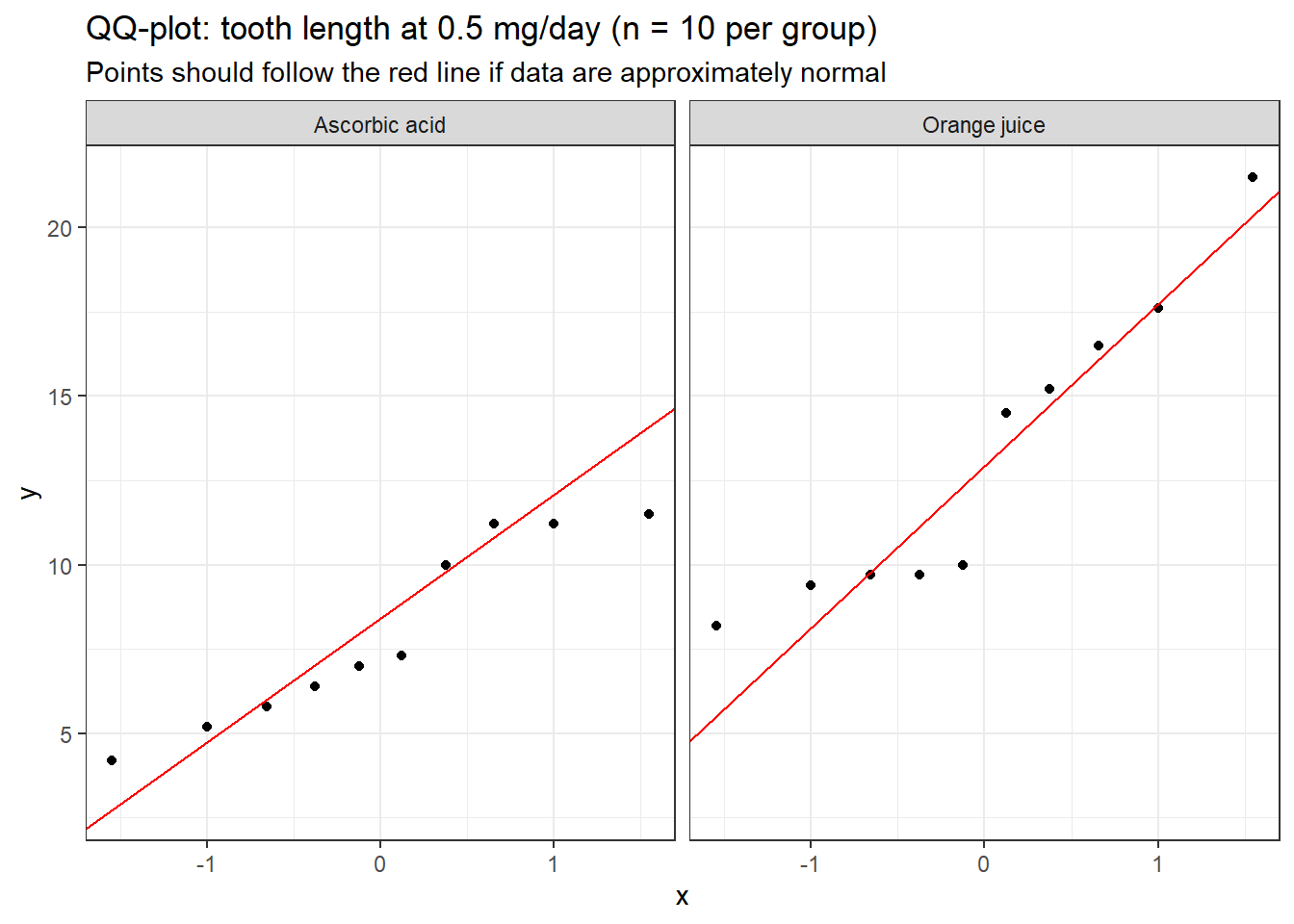
The decision between a t-test and a Wilcoxon test should be made before running the test, based on a QQ-plot and the sample size. Here we demonstrate this decision with ToothGrowth at the 0.5 mg/day dose where each group has only 10 guinea pigs.
tg_05 <- ToothGrowth %>%as_tibble() %>%mutate(supp =factor(supp, levels =c("VC", "OJ"),labels =c("Ascorbic acid", "Orange juice")) ) %>%filter(dose ==0.5)tg_05 %>%ggplot(aes(sample = len)) +stat_qq() +stat_qq_line(colour ="red") +facet_wrap(~supp) +labs(title ="QQ-plot: tooth length at 0.5 mg/day (n = 10 per group)",subtitle ="Points should follow the red line if data are approximately normal" ) +theme_bw()
With n = 10 and some departure from the line, the Wilcoxon test is the safer choice here. The t-test would also be defensible (the deviations are not severe), but when in doubt with small samples, use the nonparametric option.
6.4.2 Two-sample Wilcoxon rank-sum test
res_wilcox <-wilcox.test(len ~ supp, data = tg_05, exact =FALSE)tidy(res_wilcox)
# A tibble: 1 × 4
  statistic p.value method                                           alternative
      <dbl>   <dbl> <chr>                                            <chr>
1      19.5  0.0232 Wilcoxon rank sum test with continuity correcti… two.sided
# A tibble: 2 × 5
  supp              n median    q1    q3
  <fct>         <int>  <dbl> <dbl> <dbl>
1 Ascorbic acid    10   7.15  5.95  10.9
2 Orange juice     10  12.2   9.7   16.2
TipRun It Yourself
Run the chunk above. You should get W ≈ 19.5 and p ≈ 0.023. The group medians are 7.15 (IQR: 5.95–10.9) for ascorbic acid and 12.2 (IQR: 9.7–16.2) for orange juice — orange juice produces longer teeth at this dose, and the gap is large relative to the spread. Before moving on, predict: will the t-test on the same data (next chunk) reach the same conclusion?
NoteReading the Wilcoxon Output
Output
What it means
statistic (W)
The sum of ranks in the first group. A large W means the first group tends to have higher values.
p.value
The probability of observing a rank distribution this extreme if both groups came from the same population.
Always report medians and IQR, not means and SD, alongside a Wilcoxon test. The test is based on ranks, so the rank-based summary (median) is the appropriate measure of location.
How does this compare to using the t-test on the same data?
Run the chunk above. The Welch t-test gives t ≈ -3.17, p ≈ 0.006, and the Wilcoxon gives W ≈ 19.5, p ≈ 0.023. Both are well below 0.05, so both tests agree: orange juice produces significantly longer teeth than ascorbic acid at this dose.
Both reach the same conclusion here. They often agree. When they disagree, trust the Wilcoxon for small non-normal samples, and investigate why they differ (usually an outlier is driving the t-test result).
6.4.3 Paired Wilcoxon signed-rank test
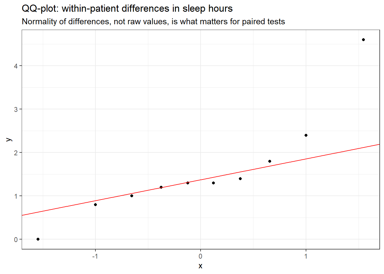
The sleep dataset has 10 patients measured under two drugs: a paired design. For the paired Wilcoxon, what matters is the normality of the within-patient differences, not the raw values.
sleepdat <- sleep %>%as_tibble() %>%rename(drug = group, extra_hours = extra) %>%mutate(drug =factor(drug, labels =c("Drug 1", "Drug 2")))sleep_wide <- sleepdat %>% tidyr::pivot_wider(names_from = drug,values_from = extra_hours,id_cols = ID )diffs <- sleep_wide[["Drug 2"]] - sleep_wide[["Drug 1"]]tibble(diff = diffs) %>%ggplot(aes(sample = diff)) +stat_qq() +stat_qq_line(colour ="red") +labs(title ="QQ-plot: within-patient differences in sleep hours",subtitle ="Normality of differences, not raw values, is what matters for paired tests" ) +theme_bw()
Warning in wilcox.test.default(sleep_wide[["Drug 2"]], sleep_wide[["Drug 1"]],
: cannot compute exact p-value with ties
Warning in wilcox.test.default(sleep_wide[["Drug 2"]], sleep_wide[["Drug 1"]],
: cannot compute exact p-value with zeroes
tidy(res_sleep)
# A tibble: 1 × 4
  statistic p.value method                                           alternative
      <dbl>   <dbl> <chr>                                            <chr>
1        45 0.00909 Wilcoxon signed rank test with continuity corre… two.sided
TipRun It Yourself
Run the chunk above (you’ll see two warnings about ties and zeroes — these are expected with small integer-valued data and do not invalidate the test). You should get V ≈ 45 and p ≈ 0.009. This is well below 0.05: Drug 2 gives significantly more extra sleep than Drug 1.
With n = 10 differences, the QQ-plot shows reasonable normality: a paired t-test would also be valid. The Wilcoxon and t-test conclusions agree here, which is reassuring.
6.5 Example 2: Clinical Data (PBC)
Estimated time: ~25 minutes (worked example)
NoteTeacher Note
The PBC dataset has been used for treatment-group comparisons in T-tests and Hypothesis Testing with albumin (a roughly symmetric variable, no significant difference between groups). Here we switch to bilirubin, which is heavily skewed in the opposite direction: ask the room why the same randomised comparison (D-penicillamine vs placebo) might call for a different test depending on which variable you look at.
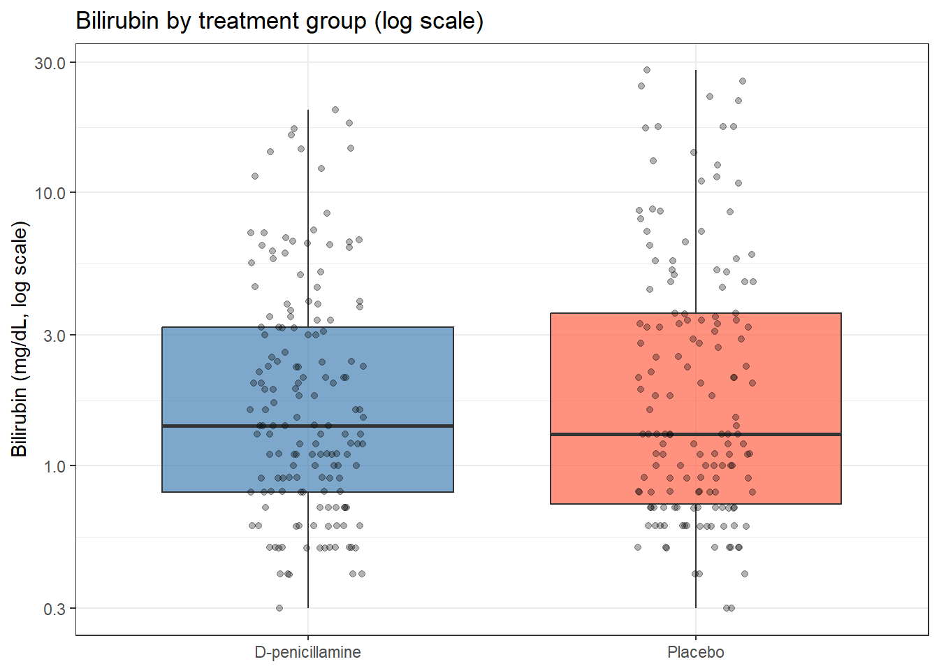
Bilirubin in the PBC dataset is a genuine case for nonparametric tests: heavily right-skewed, extreme outliers, and meaningful biological variability. No log transformation changes the underlying problem: the distribution is better described by its median and spread than its mean.
# A tibble: 1 × 4
  statistic p.value method                                           alternative
      <dbl>   <dbl> <chr>                                            <chr>
1     12007   0.842 Wilcoxon rank sum test with continuity correcti… two.sided
# A tibble: 2 × 5
  trt                 n median    q1    q3
  <fct>           <int>  <dbl> <dbl> <dbl>
1 D-penicillamine   158    1.4 0.8     3.2
2 Placebo           154    1.3 0.725   3.6
TipRun It Yourself
Run the chunk above. You should get W ≈ 12007 and p ≈ 0.84. The medians are 1.4 mg/dL (IQR: 0.8–3.2, n = 158) for D-penicillamine and 1.3 mg/dL (IQR: 0.725–3.6, n = 154) for placebo — very similar distributions, as expected for a randomised baseline comparison.
No significant difference at baseline (median bilirubin 1.4 mg/dL, IQR: 0.8–3.2, in the D-penicillamine group vs 1.3 mg/dL, IQR: 0.725–3.6, in the placebo group; Wilcoxon rank-sum: W = 12007, p = 0.84), consistent with successful randomisation.
6.5.2 Kruskal-Wallis: three or more groups
The Kruskal-Wallis test is the nonparametric analogue of one-way ANOVA. It tests whether at least one group differs from the others, but does not tell you which pairs differ. A significant result requires post-hoc pairwise comparisons with multiple testing correction.
Does bilirubin differ across the four disease stages?
pbc_stage <- pbc %>%filter(!is.na(stage), !is.na(bili))kruskal.test(bili ~ stage, data = pbc_stage)
    Kruskal-Wallis rank sum test

data:  bili by stage
Kruskal-Wallis chi-squared = 46.638, df = 3, p-value = 4.15e-10
TipRun It Yourself
Run the chunk above. You should get chi-squared ≈ 46.6, df = 3, and p ≈ 4e-10 — a tiny p-value, far below 0.05. At least one disease stage differs from the others in bilirubin.
The overall test is highly significant: bilirubin clearly rises with disease stage, as expected biologically. Now identify which specific stage pairs account for this:
    Pairwise comparisons using Wilcoxon rank sum test with continuity correction

data:  pbc_stage$bili and pbc_stage$stage

        Stage 1 Stage 2 Stage 3
Stage 2 1.000   -       -
Stage 3 0.029   0.168   -
Stage 4 2.0e-05 2.1e-07 8.1e-05

P value adjustment method: bonferroni
TipRun It Yourself
Run the chunk above. You should get a table of pairwise p-values. Stage 1 vs Stage 2 (p = 1.000) and Stage 2 vs Stage 3 (p = 0.168) are not significant after Bonferroni correction, and Stage 1 vs Stage 3 is borderline (p = 0.029). Every comparison involving Stage 4 is highly significant (p < 0.0001). In words: bilirubin in Stage 4 is clearly different from every earlier stage, while the early stages are harder to tell apart from each other.
The post-hoc table shows which stage pairs are significantly different after Bonferroni correction. Early stages (1 and 2) tend not to differ from each other, but later stages (3 and 4) separate clearly.
NoteAfter Kruskal-Wallis: what to report
A significant Kruskal-Wallis result tells you “at least one group differs.” To say more, you need post-hoc pairwise tests. Always apply a multiple testing correction ("bonferroni" is conservative but clear; "holm" is slightly more powerful). Report the overall test result and then summarise which pairs differed.
6.6 What Can Go Wrong
Estimated time: ~10 minutes (reading)
NoteTeacher Note
Run a quick true/false round on the “Common misinterpretations” callout below: read each bold statement aloud and ask for a thumbs up/down before revealing the explanation. The “Wilcoxon makes no assumptions” one is usually the most surprising to students who learned it as “the test you use when you can’t make assumptions.”
Using nonparametric tests as the default “safe” choice
Nonparametric tests are not always better. When data are approximately normal, the t-test is more powerful: it extracts more information from the same data. Switching to nonparametric by default when a t-test would be valid is a quiet way to reduce your power to detect real effects. Make the decision from the data: check the QQ-plot and the sample size.
Reporting means alongside a Wilcoxon result
The Wilcoxon test is based on ranks, which correspond to the median as a measure of location. If you report means and SDs in your results table and then cite a Wilcoxon p-value in the text, you are mixing incompatible summaries. Report medians and IQR when using nonparametric tests.
Skipping post-hoc correction after Kruskal-Wallis
Running six pairwise Wilcoxon tests without correction after a Kruskal-Wallis gives a false positive rate far above 5%. Always specify a correction method in pairwise.wilcox.test().
Interpreting a non-significant result as “no difference”
With small samples, nonparametric tests have limited power. A p > 0.05 from a Wilcoxon test with n = 8 per group means you could not detect a difference, not that no difference exists. Report the medians, IQR, and sample size so readers can judge whether the study was adequately powered.
WarningCommon misinterpretations
“Nonparametric tests make no assumptions” They do. The Wilcoxon rank-sum test assumes the two distributions have the same shape and only differ in location (shift). It is more robust than the t-test, but not assumption-free.
“I used a Wilcoxon test because my data failed Shapiro-Wilk” Shapiro-Wilk is a poor decision tool (see T-tests). Use a QQ-plot and your knowledge of the outcome instead. If bilirubin is right-skewed in every study ever published, you do not need a formal normality test to justify a Wilcoxon.
“The Wilcoxon test compares medians” Not exactly. It tests whether one group’s values tend to be larger than the other’s: technically, whether P(X > Y) = 0.5. This is close to comparing medians when the distributions have the same shape, but not in general.
6.7 Exercises
NoteTeacher Note
Pair students for Exercises 1 and 2: one person runs the code while the other predicts the result before each output appears (medians, then test statistic, then p-value). Exercise 1 has a genuine surprise in store (see the solution), which works best if students commit to a prediction first.
6.7.1 Exercise 1 (Guided): Wilcoxon Test for Bilirubin by Sex
Estimated time: ~15 minutes
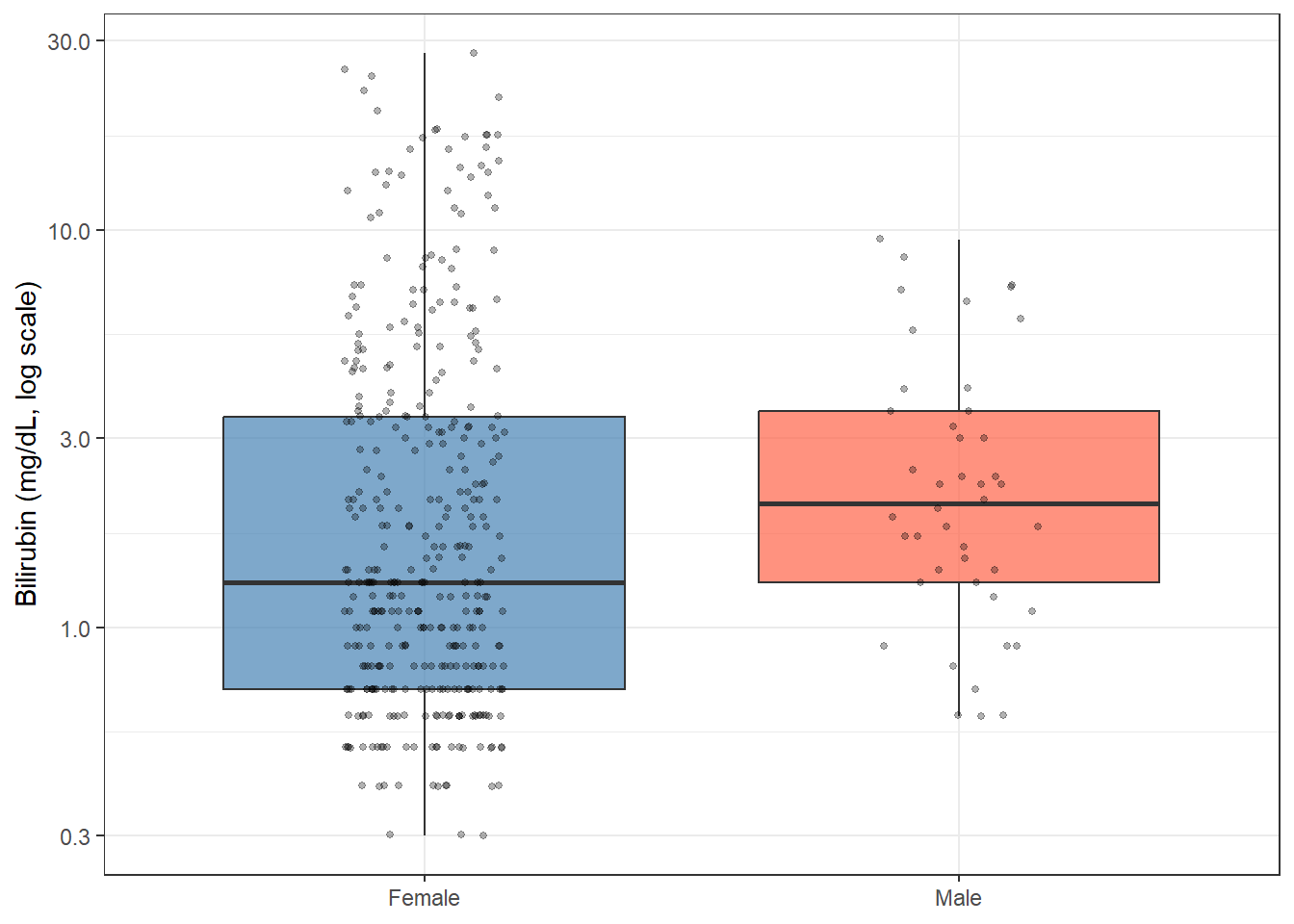
Using survival::pbc, test whether bilirubin differs between male and female patients.
Plot bilirubin by sex using a log scale on the y-axis.
Compute medians and IQR for each sex.
Run a Wilcoxon rank-sum test.
For comparison, run a t-test on log(bili). Do both tests reach the same conclusion?
# A tibble: 2 × 5
  sex        n median    q1    q3
  <fct>  <int>  <dbl> <dbl> <dbl>
1 Female   374   1.3    0.7   3.4
2 Male      44   2.05   1.3   3.5
tidy(wilcox.test(bili ~ sex, data = pbc_sex))
# A tibble: 1 × 4
  statistic p.value method                                           alternative
      <dbl>   <dbl> <chr>                                            <chr>
1     6574.  0.0290 Wilcoxon rank sum test with continuity correcti… two.sided
Run the chunk above. Median bilirubin is 1.3 mg/dL (IQR: 0.7–3.4) for females (n = 374) and 2.05 mg/dL (IQR: 1.3–3.5) for males (n = 44). The Wilcoxon test gives W ≈ 6574, p ≈ 0.029 — significant at the 0.05 level. But the t-test on log(bili) gives t ≈ -1.73, df ≈ 64, p ≈ 0.089 — not significant.
This time the two tests disagree: the Wilcoxon says males and females differ significantly, the t-test on log-bilirubin does not quite reach 0.05. This is a useful real example, not an error. A few things are happening at once: the male group is small (n = 44) and the two group sizes are very unequal (44 vs 374), which affects the t-test’s power and its degrees of freedom (Welch’s correction gives df ≈ 64, far below the 416 you might naively expect). The Wilcoxon, working on ranks across the whole sample, is less sensitive to that imbalance here. When two reasonable methods disagree like this, do not pick whichever gives the answer you want — report both results and let the reader judge, or note that the result is borderline and would benefit from a larger male sample.
6.7.2 Exercise 2 (Semi-guided): Kruskal-Wallis Across Disease Stages
Estimated time: ~15 minutes
Test whether bilirubin differs across disease stages 1–4 in pbc.
Run kruskal.test(). Is the overall test significant?
Run pairwise.wilcox.test() with Bonferroni correction. Which stage pairs are significantly different?
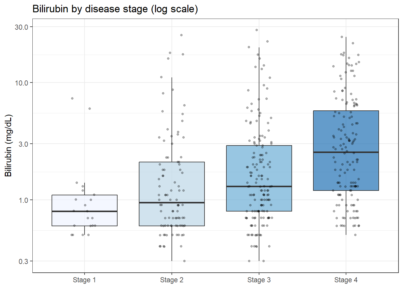
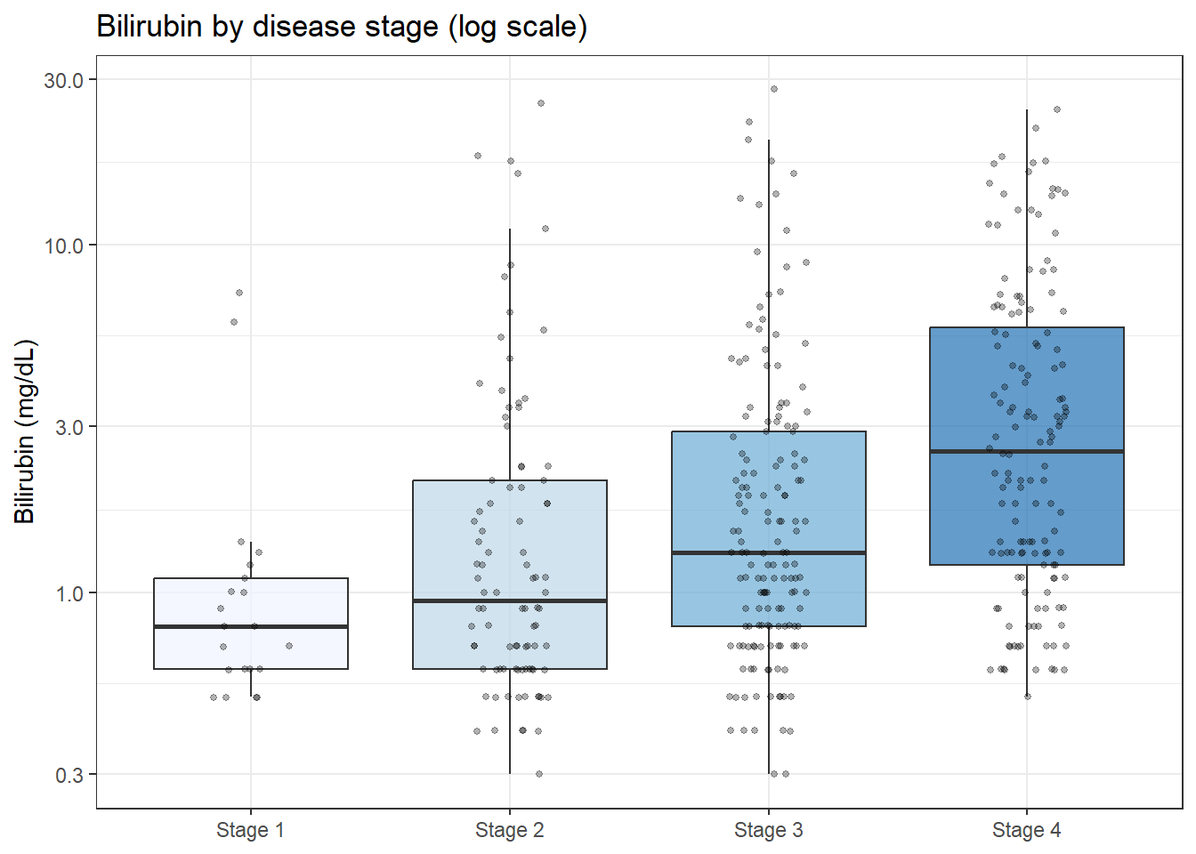
Create a boxplot (log scale) to visualise the pattern.
Does the pattern make biological sense? What would you expect for a progressive disease?
TipExercise 2: Solution
pbc_s <- pbc %>%filter(!is.na(stage), !is.na(bili))kruskal.test(bili ~ stage, data = pbc_s)
    Kruskal-Wallis rank sum test

data:  bili by stage
Kruskal-Wallis chi-squared = 46.638, df = 3, p-value = 4.15e-10
    Pairwise comparisons using Wilcoxon rank sum test with continuity correction

data:  pbc_s$bili and pbc_s$stage

        Stage 1 Stage 2 Stage 3
Stage 2 1.000   -       -
Stage 3 0.029   0.168   -
Stage 4 2.0e-05 2.1e-07 8.1e-05

P value adjustment method: bonferroni
pbc_s %>%ggplot(aes(x = stage, y = bili, fill = stage)) +geom_boxplot(alpha =0.7, outlier.shape =NA) +geom_jitter(width =0.15, alpha =0.3, size =1) +scale_fill_brewer(palette ="Blues") +scale_y_log10() +labs(title ="Bilirubin by disease stage (log scale)",x =NULL, y ="Bilirubin (mg/dL)" ) +theme_bw() +theme(legend.position ="none")
For a progressive disease, we expect bilirubin to rise with stage, and it does. The pairwise tests show that adjacent early stages may not differ significantly, but the gap between early and late stages is substantial and highly significant.
6.7.3 Exercise 3 (Open-ended)
Estimated time: 15–30 minutes
From your own data, find a continuous variable that is clearly non-normal (cytokine levels, viral load, cell counts, enzyme concentrations). Run both a t-test and a Wilcoxon test on the same comparison. Do they agree? If they disagree, investigate why: look at the data and identify what is driving the difference.
6.8 Comprehension Check
Estimated time: ~10 minutes (self-test)
In what two situations is a nonparametric test preferred over a t-test?
What does it mean to “test on ranks”? Give a concrete example of why this makes a test robust to outliers.
You run a Kruskal-Wallis test and get p = 0.02 across four groups. What should you do next?
You used a Wilcoxon test. Should you report means or medians in your results table?
A colleague says “I always use Wilcoxon because it doesn’t assume normality, so it’s safer.” Is this a good strategy?
NoteAnswers
When (1) sample size is small (\(n < 30\) per group) and data are visibly non-normal on a QQ-plot, or (2) the outcome has extreme outliers that represent real biology rather than measurement error. Also appropriate for ordinal outcomes.
All observations are ranked from smallest to largest, and the test compares the distribution of ranks between groups rather than the raw values. Example: values of 1, 3, 5, 7, 42 become ranks 1, 2, 3, 4, 5. Changing 42 to 420 does not change the ranks, so the test result is unaffected by that extreme value.
Follow up with pairwise Wilcoxon tests using pairwise.wilcox.test() with a multiple testing correction (Bonferroni or Holm). The Kruskal-Wallis result tells you “at least one group differs”; post-hoc tests identify which specific pairs.
Medians and IQR. The Wilcoxon test is based on ranks, and the median is the rank-based measure of location. Reporting means alongside a Wilcoxon result is internally inconsistent.
Not a good general strategy. When data are approximately normal, the t-test is more powerful. Using Wilcoxon by default costs statistical power unnecessarily. Make the decision based on the QQ-plot and sample size, not out of caution.
6.9 How to Report
NoteReporting Nonparametric Results
In a Methods section:
“Because [outcome] was markedly right-skewed with extreme outliers (confirmed by QQ-plot), the Wilcoxon rank-sum test was used to compare groups and results are presented as median (IQR). For comparisons across three or more groups, the Kruskal-Wallis test was used, followed by pairwise Wilcoxon tests with Bonferroni correction.”
In a Results section:
“Median [outcome] was X (IQR: A–B) in [group 1] and Y (IQR: C–D) in [group 2]; groups did not differ significantly (Wilcoxon rank-sum: W = Z, p = P).”
“Bilirubin differed significantly across disease stages (Kruskal- Wallis: H(3) = XX.X, p < 0.001). Post-hoc pairwise comparisons with Bonferroni correction showed significant differences between Stages 1 and 4 (p = 0.001) and Stages 2 and 4 (p = 0.003).”
Always include:
Medians and IQR for each group (not means and SD)
Test statistic (W for Wilcoxon, H for Kruskal-Wallis with df)
Exact p-value
Post-hoc method and correction when multiple comparisons are made
6.10 Further Reading
Bland (2015): An Introduction to Medical Statistics: clear chapters on nonparametric methods written for clinicians
Hollander and Wolfe (1999): Nonparametric Statistical Methods: comprehensive reference
?wilcox.test and ?kruskal.test in R: built-in help with worked examples
Bland, Martin. 2015. An Introduction to Medical Statistics. 4th ed. Oxford University Press.
Hollander, Myles, and Douglas A. Wolfe. 1999. Nonparametric Statistical Methods. 2nd ed. John Wiley & Sons.