Total core time: ~155 minutes (about 2.5 hours). A natural break point is after Example 1 (drawing and querying DAGs)—cover Example 2 (propensity scores) and the exercises in a second sitting. Exercise 3 is open-ended and its time will vary.
Section
Time
Type
The Key Idea: Correlation Is Not Causation
~10 min
Concept
Background: Why Associations Are Not Causes
~15 min
Concept
Example 1: Drawing a DAG for PBC
~35 min
Walkthrough
Example 2: Propensity Score Analysis
~25 min
Walkthrough
What Can Go Wrong
~10 min
Reading
Exercise 1 (Guided)
~15 min
Practice
Exercise 2 (Semi-guided)
~15 min
Practice
Exercise 3 (Open-ended)
15–30 min
Practice
Comprehension Check
~10 min
Self-test
If you are short on time, the collider-bias demonstration in Example 1 (the collider-demo chunk) is the single most counterintuitive and memorable result in this session: a correlation of essentially zero becomes a strong spurious correlation just by restricting the sample on a shared outcome.
TipHow to Use the Code in This Session
Every code chunk below is written so you can copy it into your R console (or an R script) and run it yourself, in the order shown. Where you see a “Run It Yourself” box, stop and run the code above it before reading the explanation that follows.
18.1 When Do You Use This?
Tip
You have found a statistical association between an exposure and an outcome, but associations can arise from confounding, reverse causation, or selection bias rather than a true causal effect. Causal inference provides the framework for deciding whether an observed association reflects a genuine causal relationship, what “adjusting for confounders” really means, and why adjusting for the wrong variables can make things worse rather than better. For example: patients who take aspirin have lower bilirubin, but does aspirin reduce bilirubin, or do healthier patients simply take aspirin more often?
NoteTeacher Note
Ask learners: when building a regression model, is it ever a bad idea to add more covariates “just to be safe”? Most will say no – more adjustment feels more careful, more conservative. This session’s central goal is to overturn that intuition: whether adjusting for a variable helps or hurts depends entirely on its causal role (confounder, mediator, or collider), which a regression model cannot tell you on its own. Keep this question in mind through the collider-bias demonstration and Exercise 1.
18.2 Learning Objectives
After completing this session you will be able to:
Distinguish association from causation and explain why regression alone cannot establish causation
Draw and interpret a directed acyclic graph (DAG) for a research question
Identify confounders, mediators, and colliders from a DAG
Apply the backdoor criterion to select a valid adjustment set
Recognise and avoid collider bias and mediation bias
18.3 The Key Idea: Correlation Is Not Causation, and Adjustment Is Not Neutral
Estimated time: ~10 minutes (Concept)
You have heard “correlation is not causation” a thousand times. But causal inference makes this concrete: it gives you a framework for knowing when a correlation reflects causation, and when adjusting for a variable helps versus hurts.
The central insight: whether to adjust for a variable depends entirely on its causal role. A confounder must be adjusted for. A mediator must NOT be adjusted for (if you want the total effect). A collider must NEVER be adjusted for. Without a causal diagram, you cannot tell these apart, and getting it wrong can introduce more bias than it removes.
18.4 Background: Why Associations Are Not Causes
Estimated time: ~15 minutes (Concept)
18.4.1 Potential Outcomes Framework
For each individual \(i\), define: - \(Y_i(1)\): the outcome if they receive treatment - \(Y_i(0)\): the outcome if they do not
The individual causal effect is \(Y_i(1) - Y_i(0)\), but we can only ever observe one of these (the fundamental problem of causal inference). We estimate the average treatment effect (ATE):
\[ATE = E[Y(1) - Y(0)]\]
In an RCT, randomisation ensures that the treated and untreated groups have the same distribution of potential confounders, so the observed difference in means estimates the ATE. In observational data, we must adjust for confounders, but we need to know which variables to adjust for.
18.4.2 Directed Acyclic Graphs (DAGs)
A DAG encodes the investigator’s causal assumptions as a graph where arrows represent direct causal effects and the absence of an arrow represents the assumption of no direct effect.
Three key structures:
Structure
Diagram
Rule
Fork (confounder)
\(X \leftarrow C \rightarrow Y\)
Adjust for \(C\) to block the backdoor path
Chain (mediator)
\(X \rightarrow M \rightarrow Y\)
Do not adjust for \(M\) if estimating total effect
Collider
\(X \rightarrow C \leftarrow Y\)
Do not adjust for \(C\) - this opens a path and introduces bias
18.5 Example 1: Drawing a DAG for PBC
Estimated time: ~35 minutes (Walkthrough)
NoteTeacher Note
This example has several natural stopping points for prediction:
Before running dag-pbc: sketch on paper (or whiteboard) a DAG for “does bilirubin cause low albumin in PBC, or is this confounded by disease stage?” Then compare with the DAG drawn in code.
Before running adjustment-set: ask learners to predict, from the DAG alone, what dagitty::adjustmentSets() will return for the effect of bili on albumin.
Before running collider-demo: ask learners to predict what will happen to the correlation between exercise and diet (currently ~0) once the sample is restricted to people with low BMI. Most learners predict “nothing changes” - the surprising result is the point.
18.5.1 The Research Question
Does bilirubin causally affect albumin in PBC patients, or is the association confounded by disease severity (stage)?
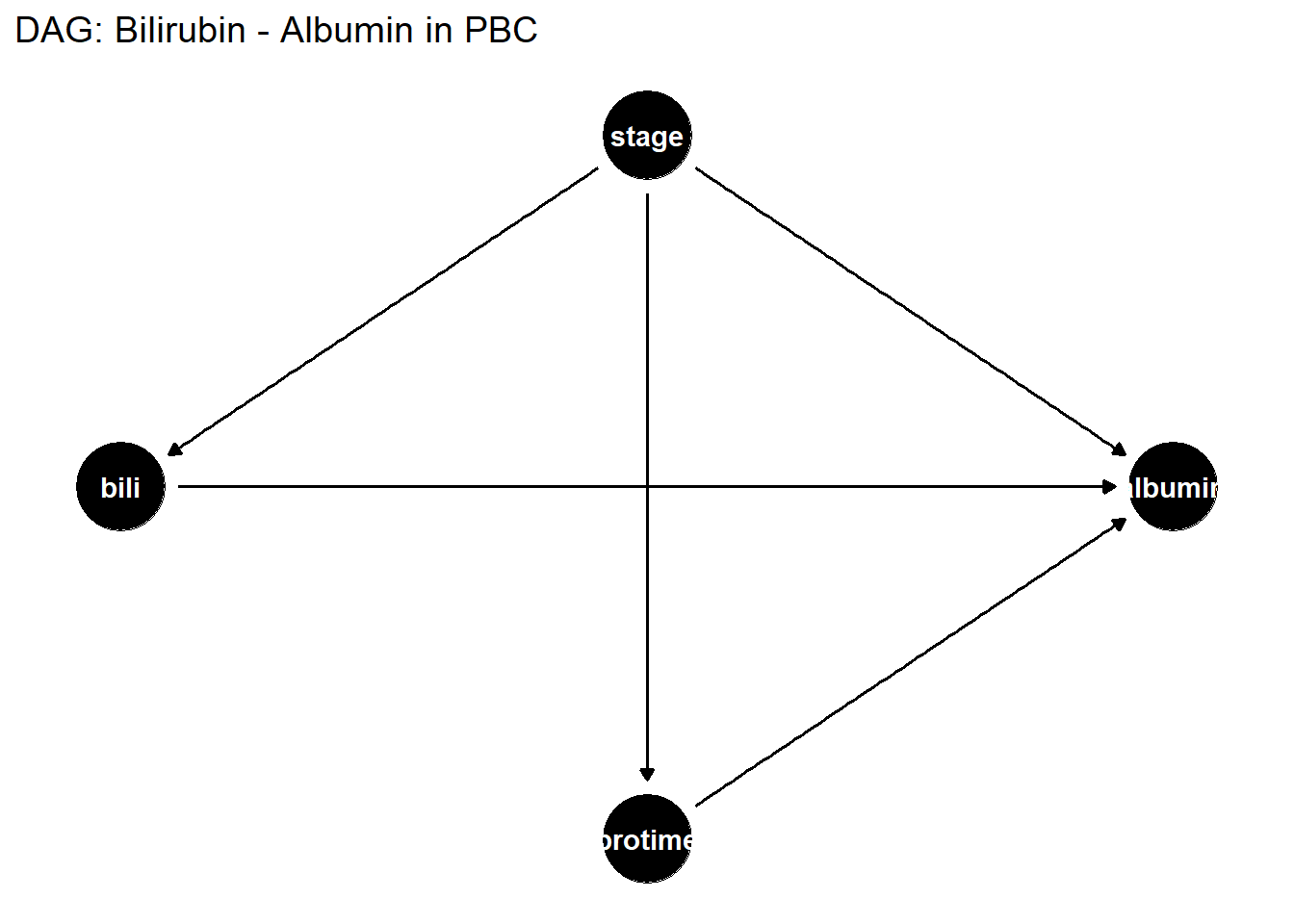
dag <- dagitty::dagitty('dag { bili -> albumin stage -> bili stage -> albumin stage -> protime protime -> albumin}')dagitty::coordinates(dag) <-list(x =c(bili =0, albumin =2, stage =1, protime =1),y =c(bili =1, albumin =1, stage =2, protime =0))ggdag::ggdag(dag, layout ="auto") +theme_dag() +labs(title ="DAG: Bilirubin - Albumin in PBC")
TipRun It Yourself
The plot shows a diamond shape: stage sits at the top with three arrows leading out to bili, albumin, and protime; bili has its own arrow into albumin; and protime also has an arrow into albumin. Visually, stage is a common cause of bili, albumin, and protime - a classic confounder structure - while protime sits between stage and albumin as well as receiving its own arrow from stage.
Before moving on: which node(s) in this DAG do you think need to be in the adjustment set if you want the causal effect of bili on albumin? Write down your answer, then check it against the next chunk.
18.5.2 Identifying the Adjustment Set
Estimated time: ~5 minutes (Walkthrough)
# What must we adjust for to estimate the causal effect of bili on albumin?dagitty::adjustmentSets(dag, exposure ="bili", outcome ="albumin")
{ stage }
TipRun It Yourself
You should see:
{ stage }
dagitty agrees with the visual reasoning: stage is the only variable you need to adjust for. protime does not need to be in the adjustment set - it lies on a path from stage to albumin that does not create a backdoor path from bili, so adjusting for it would not be necessary (and, depending on the question, could even be harmful - see the next section).
The backdoor criterion says: block all non-causal paths from bili to albumin. In this DAG, stage is a common cause (confounder) - it opens a backdoor path. Adjusting for stage closes this path.
18.5.3 What If We Adjust for a Mediator?
dag2 <- dagitty::dagitty('dag { bili -> protime protime -> albumin bili -> albumin}')dagitty::adjustmentSets(dag2, exposure ="bili", outcome ="albumin",effect ="total")
{}
TipRun It Yourself
You should see:
{}
An empty set - dagitty says you should adjust for nothing. In this DAG, protime lies entirely on the causal path from bili to albumin (a mediator), so it is not part of any backdoor path. If you adjusted for protime here, you would block part of the very effect you are trying to estimate, biasing your estimate of the total effect of bili on albumin toward zero.
If protime is on the causal pathway from bilirubin to albumin (a mediator), adjusting for it blocks part of the effect of bilirubin. We would then estimate only the direct effect, not the total effect. Be explicit about whether you want total or direct effects.
18.5.4 Collider Bias: A Demonstration
Estimated time: ~10 minutes (Walkthrough)
set.seed(2024)n <-1000# Simulate: exercise and diet both independently affect BMI# But exercise and diet are NOT associated in the populationdf <-tibble(exercise =rnorm(n),diet =rnorm(n),bmi =-0.5* exercise -0.5* diet +rnorm(n, 0, 0.5))# Unadjusted: no correlation between exercise and dietcat("r(exercise, diet) =", round(cor(df$exercise, df$diet), 3), "\n")
In the full simulated sample, exercise and diet are essentially uncorrelated (r = -0.014), exactly as we built them: independent random draws. But once we restrict to the lowest BMI quintile - conditioning on bmi, which is caused by bothexercise and diet - a strong negative correlation (r = -0.384) appears out of nowhere.
Why? Among people with very low BMI, low exercise must be “compensated for” by a stricter diet (and vice versa) to end up in that low-BMI group. The collider has manufactured a relationship between two variables that were never related in the first place. No causal link between exercise and diet was created by this restriction - the association is entirely an artefact of how the sample was selected.
Restricting to low BMI (conditioning on the collider) creates a spurious negative correlation between exercise and diet. This is collider bias - conditioning on a common effect of two variables induces an association between them.
Practical example: In a study of ICU patients, restricting the sample to those admitted to ICU (a collider of severe illness and random events) can make risk factors appear protective; this is Berkson’s paradox.
18.6 Example 2: Propensity Score Analysis
Estimated time: ~25 minutes (Walkthrough)
NoteTeacher Note
The survival::pbc data come from a randomised trial, so treatment assignment should already be close to balanced on measured covariates. Ask learners to predict, before running iptw: do they expect the IPTW-adjusted estimate of the effect of trt_d on albumin to differ much from a simple unadjusted comparison? And how might this connect to the log-rank test result from the Survival and Time-to-Event session, which found no significant difference in survival between treatment arms (p = 0.7)?
When randomisation is not possible, propensity score methods attempt to balance confounders between treatment groups.
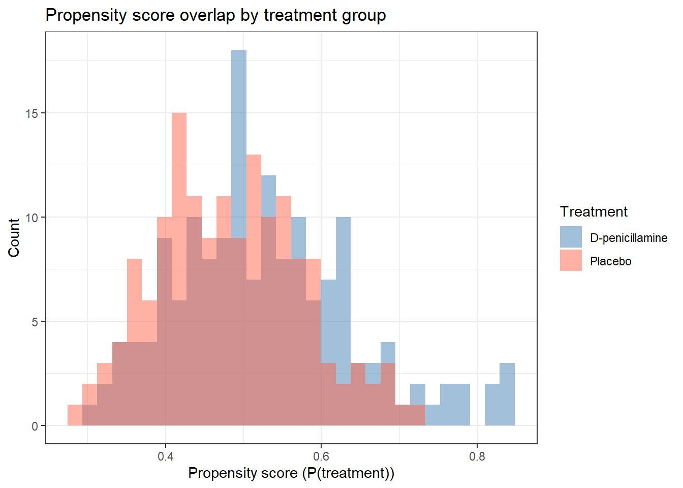
The two distributions overlap substantially across the 0.3-0.7 range, which is reassuring. However, look closely at the upper tail: the D-penicillamine group (steelblue) has additional mass out to propensity scores of 0.6-0.85, where the Placebo group (tomato) has little or no presence. This is a mild positivity concern - for patients whose covariates put them at the high end of this range, we have few or no observed Placebo patients to compare against, so any IPTW estimate in that region relies more heavily on extrapolation (and those patients will receive large weights if they are in the Placebo group).
Good overlap (positivity) is required for propensity score methods to work. If the groups are completely separated on the propensity score, there is no common support; the causal question cannot be answered from these data alone.
After IPTW adjustment, the estimated effect of D-penicillamine versus placebo on albumin is essentially zero (0.003 g/dL, 95% CI -0.09 to 0.10, p = 0.946). This matches the prediction from the Teacher Note: since pbc comes from a randomised trial, treatment groups were already well-balanced before weighting, and the log-rank test in the Survival and Time-to-Event session likewise found no significant survival difference between arms (p = 0.7). Two different outcomes (albumin and survival), two different methods (IPTW-weighted regression and the log-rank test), and the same conclusion: this trial found no detectable benefit of D-penicillamine.
IPTW creates a pseudo-population in which treatment assignment is independent of confounders. The weighted outcome difference estimates the ATE.
NoteWhere to Find Data Like This
survival::pbc: Real RCT data: bilirubin, albumin, stage, prothrombin time, ideal for DAG-based confounding analysis.
dagitty.net: Free online DAG tool: draw, encode, and query adjustment sets without R.
ggdag and dagitty R packages: Programmatic DAG construction, visualisation, and adjustment set identification.
WarningWhat Can Go Wrong
Estimated time: ~10 minutes (Reading)
Adjusting for everything. Adding all available variables to a regression model is not “conservative”: it can introduce collider bias if any of those variables is a collider. Always draw a DAG before deciding what to adjust for.
Over-adjusting for mediators. If you adjust for a mediator, you estimate the direct effect of exposure on outcome. This is only correct if your research question specifically asks about the direct effect. For most aetiological questions, you want the total effect, which means not adjusting for mediators.
Confusing statistical control with causal identification. A regression coefficient “adjusted for X” does not automatically equal the causal effect. The causal interpretation requires the DAG-based assumptions to hold: no unmeasured confounders, correct functional form, no measurement error in confounders.
Positivity violations in propensity score methods. If some patient subgroups always or never receive treatment, inverse probability weights become extreme or undefined. Trim weights or restrict the analysis to the region of common support.
18.7 Exercises
NoteTeacher Note
Exercise 1 mirrors the mediator example from earlier in this session (dag-mediator), but applied to a new question: the effect of stage on died, with albumin and bili as intermediate variables. Before learners run the solution code, ask them to predict whether the adjustment set will be empty, contain albumin, or contain something else - and to articulate why based on the causal roles (confounder vs. mediator) of each variable.
18.7.1 Exercise 1 (Guided): Draw and Query a DAG
Estimated time: ~15 minutes (Practice)
Consider this question: “Does albumin mediate the effect of disease stage on mortality in PBC?”
Draw a DAG with nodes: stage, albumin, bili, died. Include arrows based on your biological knowledge.
Use dagitty::adjustmentSets() to find what to adjust for when estimating the effect of stage on died (total effect).
Is albumin a mediator, confounder, or collider in this DAG?
TipExercise 1: Solution
dag_ex <- dagitty::dagitty('dag { stage -> albumin stage -> bili stage -> died albumin -> died bili -> albumin bili -> died}')dagitty::adjustmentSets(dag_ex, exposure ="stage", outcome ="died",effect ="total")
{}
# albumin is a mediator (stage -> albumin -> died)# adjusting for albumin would block part of the total effect
adjustmentSets() returns {} - an empty set, meaning you should adjust for nothing to estimate the total effect of stage on died. albumin is a mediator: it lies on the causal pathway stage -> albumin -> died. Adjusting for it would block part of the very effect we want to measure, biasing the total-effect estimate toward zero. bili is also a mediator here (stage -> bili -> albumin -> died and stage -> bili -> died), so it too should be left out of the adjustment set for a total-effect analysis.
Using the pbc dataset and the propensity score model fitted above:
Check covariate balance before and after weighting: compare mean log_bili, albumin, log_proto between treatment groups in the raw data and in the IPTW-weighted data.
Is balance achieved? What is the standardised mean difference for log_bili before and after weighting?
TipExercise 2: Solution
# Raw SMDsmd <-function(x, treat) { d <-mean(x[treat ==1]) -mean(x[treat ==0]) s <-sqrt((var(x[treat ==1]) +var(x[treat ==0])) /2) d / s}cat("Raw SMD log_bili:", round(smd(pbc$log_bili, pbc$trt_d), 3), "\n")
Raw SMD log_bili: -0.074
Weighted SMD log_bili: -0.011
Both values are small (well under the common rule-of-thumb threshold of 0.1), so log_bili is reasonably balanced between treatment groups even before weighting - as expected in a randomised trial. IPTW weighting reduces the imbalance further, from -0.074 to -0.011. This illustrates two things: (1) even RCT data has small non-zero raw imbalances on individual covariates due to sampling variation, and (2) IPTW can improve balance on measured covariates, but - as in this example - it has little left to do when the data are already well balanced.
18.7.3 Exercise 3 (Open-ended)
Estimated time: 15–30 minutes (Practice)
For your own observational research question: 1. Draw a DAG encoding your assumptions about the data-generating process. 2. Use dagitty::adjustmentSets() to identify the minimal sufficient adjustment set. 3. Check whether any of your standard covariates might be colliders or mediators. 4. Write a Causal Assumptions section for your Methods, describing the DAG and justifying each arrow.
18.8 Comprehension Check
Estimated time: ~10 minutes (Self-test)
You adjust for 15 variables in a regression “to be safe.” Why might this make your causal estimate worse?
You restrict your analysis to hospitalised patients to reduce confounding by severity. A colleague says this introduces collider bias. Explain why.
You want the total effect of bilirubin on mortality. Should you adjust for albumin if albumin is on the causal pathway? Why?
Propensity scores are estimated from a logistic model. You get an AUC of 0.95. Is this good for IPTW?
The treatment effect from an RCT is -0.3 g/dL for albumin. Your observational IPTW estimate is -0.05 g/dL. What might explain the discrepancy?
NoteAnswers
Adjusting for a collider opens a backdoor path that was previously closed, inducing a spurious association. Adjusting for a mediator removes part of the causal effect, biasing toward the null. Without a DAG, you cannot know whether your covariates are confounders, mediators, or colliders; adding all of them can introduce more bias than it removes.
Hospitalisation is a common effect of the exposure (e.g., bilirubin) and other causes. Restricting to hospitalised patients conditions on a collider, creating a spurious association between bilirubin and those other causes within the hospitalised sample. This is Berkson’s paradox.
No; if albumin is a mediator on the causal pathway from bilirubin to mortality, adjusting for it blocks that pathway and estimates only the direct effect of bilirubin not mediated through albumin. To estimate the total causal effect of bilirubin (including the pathway through albumin), you should not adjust for albumin.
A high AUC (0.95) for the propensity score model means treatment and control groups are almost perfectly separable based on covariates. This is actually problematic for IPTW: patients near the boundary of the score distribution will have extreme weights (very high or very low), causing instability and high variance. Good overlap is signalled by a moderate AUC (0.6–0.8). With AUC = 0.95 you should check for positivity violations and consider weight trimming.
Several explanations: (1) Unmeasured confounding: IPTW only adjusts for measured covariates; if key confounders are unmeasured, the observational estimate is biased. (2) Selection bias - the RCT may have enrolled a different population. (3) Non-adherence in the RCT - the -0.3 is an intention-to-treat estimate, potentially diluted by non-compliance. (4) Positivity violations in the IPTW analysis leading to biased estimation. Comparing RCT and observational estimates is a useful internal validity check.
18.9 How to Report
NoteReporting a Causal Analysis
In a Methods section:
“We used a directed acyclic graph (DAG) to identify confounders and determine the minimal sufficient adjustment set for estimating the effect of [exposure] on [outcome]. The DAG was constructed using dagitty (Textor et al., 2016). Confounders identified from the DAG were included as covariates in a multivariable [regression model type], yielding an adjusted [odds ratio / hazard ratio / coefficient] for [exposure].”
In a Results section:
“After adjustment for [list covariates from DAG], the association between [exposure] and [outcome] was [direction and magnitude]: adjusted OR = X.XX (95% CI: L.LL-U.UU, p = .YYY). The unadjusted association was OR = X.XX, suggesting [direction] confounding by [confounder(s)].”
Always report: - What confounders were adjusted for, and how they were identified (ideally via a DAG) - Both unadjusted and adjusted estimates (so readers can see the direction of confounding) - That mediators and colliders were not adjusted for (if relevant)
Common reporting errors: - Adjusting for all available covariates regardless of causal structure: this can introduce collider bias - Adjusting for mediators on the causal path: this blocks the effect you are trying to estimate - Describing a result as “causal” when it is observational without instrumental variable or experimental design
18.10 Further Reading
Hernan and Robins (2023): Causal Inference: What If (free PDF: causalinferencebook.net)
Pearl (2009): Causality: Models, Reasoning, and Inference
dagitty package and website (dagitty.net) for interactive DAG construction
VanderWeele (2015): Explanation in Causal Inference - mediation analysis