12  Multiple Linear Regression

ImportantBefore You Start

This session extends simple linear regression to multiple predictors. If you have not done so yet, complete the Linear Regression session first.

NoteSession at a Glance

Total core time: ~135 minutes, plus exercises.

Section	Time	Type
When Do You Use This? + Learning Objectives	~5 min	reading
The Key Idea: Adjusting for Confounders	~10 min	reading/discussion
Background: Extending the Linear Model	~15 min	reading
Example 1: Clinical Data (PBC)	~40 min	code-along
Example 2: Animal Data (palmerpenguins)	~15 min	code-along
What Can Go Wrong	~10 min	reading
Exercises 1 & 2	~30 min	guided practice
Comprehension Check	~10 min	self-test

Example 1 is the longest section in this session, since it covers model building, multicollinearity, model comparison, and interactions in one worked example. If you are short on time, you can stop after “Checking for Multicollinearity” and treat the LRT and interaction subsections as optional. Exercise 3 is open-ended and can be assigned as take-home work.

TipHow to Use the Code in This Session

Every code chunk below is written so you can copy it into your R console (or an R script) and run it yourself, in the order shown. Where you see a “Run It Yourself” box, stop and run the code above it before reading the explanation that follows.

12.1 When Do You Use This?

Tip

You have a continuous outcome and multiple predictors, some of which are correlated with each other. Multiple regression estimates each predictor’s independent effect, holding the others constant, so you can adjust for confounders and identify which variables have a genuine association with the outcome. For example: estimating the effect of bilirubin on albumin after accounting for prothrombin time and disease stage.

NoteTeacher Note

Ask the room to recall the Linear Regression session’s bilirubin-albumin example (slope ≈ −0.14, R² ≈ 0.12). Ask: “If we also adjust for prothrombin time and disease stage, do you expect the bilirubin coefficient to get bigger, smaller, or stay about the same?” Most learners will guess “smaller” once reminded that bilirubin, prothrombin time, and stage are all correlated measures of liver function – this sets up the confounding-adjustment story in Example 1.

12.2 Learning Objectives

After completing this session you will be able to:

• Build a multiple linear regression model with continuous and categorical predictors
• Interpret coefficients as partial effects adjusted for other predictors
• Detect and handle multicollinearity using VIF
• Compare nested models using AIC and likelihood ratio tests
• Interpret and report interaction terms

12.3 The Key Idea: Adjusting for Confounders

Estimated time: ~10 minutes (reading/discussion)

Imagine you find that people who carry lighters have higher rates of lung cancer. Does carrying a lighter cause lung cancer? No, both carrying a lighter and lung cancer are caused by a shared variable: smoking. Smoking is a confounder.

Multiple regression handles this by estimating the effect of each predictor while holding the others fixed. The coefficient for “lighter-carrying” in a model that includes smoking status will shrink dramatically, because we have accounted for the shared cause.

Every coefficient in a multiple regression model answers the question: “what is the relationship between this predictor and the outcome, among people who are otherwise comparable on all the other predictors in the model?”

12.4 Background: Extending the Linear Model

Estimated time: ~15 minutes (reading)

A multiple regression with \(p\) predictors is:

\[Y_i = \beta_0 + \beta_1 X_{1i} + \beta_2 X_{2i} + \cdots + \beta_p X_{pi} + \varepsilon_i\]

Each \(\beta_j\) is the partial effect of \(X_j\) on \(Y\), holding all other predictors constant. This is what allows confounding adjustment.

Categorical predictors are included as dummy variables. R creates them automatically from factors: one level becomes the reference, and the other levels get their own coefficient representing the difference from the reference.

Interactions allow the effect of one predictor to depend on another:

\[Y = \beta_0 + \beta_1 X_1 + \beta_2 X_2 + \beta_3 (X_1 \times X_2) + \varepsilon\]

Multicollinearity: When predictors are highly correlated, their coefficients become unstable. Variance Inflation Factor (VIF) > 5–10 signals a problem.

12.5 Example 1: Clinical Data (PBC)

Estimated time: ~40 minutes (code-along)

NoteTeacher Note

This example has several moving parts: model building, coefficient interpretation, VIF, a likelihood ratio test, and an interaction. If running this live, consider pacing it as four short stops rather than one long block: (1) fit and compare the four models, (2) interpret the full model’s coefficients, (3) VIF + LRT, (4) the interaction. Each stop has its own “Run It Yourself” box below.

12.5.1 Build a Multivariable Model

We predict albumin from bilirubin, prothrombin time, and disease stage.

pbc <- survival::pbc %>%
  as_tibble() %>%
  clean_names() %>%
  filter(!is.na(albumin), !is.na(bili), !is.na(protime), !is.na(stage)) %>%
  mutate(
    log_bili   = log(bili),
    log_proto  = log(protime),
    stage      = factor(stage, levels = 1:4, labels = paste("Stage", 1:4))
  )

fit1 <- lm(albumin ~ log_bili,  data = pbc)
fit2 <- lm(albumin ~ log_proto, data = pbc)
fit3 <- lm(albumin ~ stage,     data = pbc)

fit_full <- lm(albumin ~ log_bili + log_proto + stage, data = pbc)
tidy(fit_full, conf.int = TRUE)

# A tibble: 6 × 7
  term         estimate std.error statistic  p.value conf.low conf.high
  <chr>           <dbl>     <dbl>     <dbl>    <dbl>    <dbl>     <dbl>
1 (Intercept)     4.41     0.557       7.92 2.25e-14    3.32     5.50  
2 log_bili       -0.107    0.0201     -5.31 1.80e- 7   -0.146   -0.0671
3 log_proto      -0.283    0.232      -1.22 2.23e- 1   -0.740    0.173 
4 stageStage 2   -0.111    0.0946     -1.18 2.41e- 1   -0.297    0.0748
5 stageStage 3   -0.103    0.0916     -1.13 2.60e- 1   -0.284    0.0767
6 stageStage 4   -0.320    0.0934     -3.42 6.80e- 4   -0.503   -0.136 

TipRun It Yourself

Run the chunk above. In fit_full, log_bili has estimate ≈ −0.107 (95% CI: −0.146 to −0.067, p < 0.001) and stageStage 4 has estimate ≈ −0.320 (95% CI: −0.503 to −0.136, p < 0.001). stageStage 2 and stageStage 3 are both close to zero and not statistically significant (p ≈ 0.24 and 0.26). Keep these numbers in mind for the next chunk.

bind_rows(
  glance(fit1) %>% mutate(model = "log_bili only"),
  glance(fit2) %>% mutate(model = "log_proto only"),
  glance(fit3) %>% mutate(model = "stage only"),
  glance(fit_full) %>% mutate(model = "full model")
) %>%
  select(model, r.squared, adj.r.squared, AIC, BIC)

# A tibble: 4 × 5
  model          r.squared adj.r.squared   AIC   BIC
  <chr>              <dbl>         <dbl> <dbl> <dbl>
1 log_bili only     0.124         0.122   408.  420.
2 log_proto only    0.0465        0.0441  442.  454.
3 stage only        0.123         0.116   412.  432.
4 full model        0.193         0.183   382.  410.

TipRun It Yourself

Run the chunk above. Each single-predictor model explains only a modest share of the variance (log_bili: R² ≈ 0.12; log_proto: R² ≈ 0.05; stage: R² ≈ 0.12), but the full model with all three predictors reaches R² ≈ 0.19 (adjusted R² ≈ 0.18) and has the lowest AIC (≈ 382, vs ≈ 408, 442, and 412 for the single-predictor models). Lower AIC means a better fit-to-complexity trade-off – the full model is preferred.

12.5.2 Interpreting Partial Coefficients

tidy(fit_full, conf.int = TRUE) %>%
  select(term, estimate, conf.low, conf.high, p.value) %>%
  mutate(across(where(is.numeric), \(x) round(x, 3)))

# A tibble: 6 × 5
  term         estimate conf.low conf.high p.value
  <chr>           <dbl>    <dbl>     <dbl>   <dbl>
1 (Intercept)     4.41     3.32      5.50    0    
2 log_bili       -0.107   -0.146    -0.067   0    
3 log_proto      -0.283   -0.74      0.173   0.223
4 stageStage 2   -0.111   -0.297     0.075   0.241
5 stageStage 3   -0.103   -0.284     0.077   0.26 
6 stageStage 4   -0.32    -0.503    -0.136   0.001

Reading the output:

• log_bili (−0.107): After adjusting for prothrombin time and stage, each one-unit increase in log(bilirubin) is associated with 0.11 g/dL lower albumin.
• stageStage 2 (−0.111): Stage 2 patients have 0.11 g/dL lower albumin than Stage 1 patients, after adjusting for bilirubin and prothrombin time – though with p ≈ 0.24, this difference is not statistically significant.

The coefficients change from the simple models because predictors share variance. Comparing univariable and multivariable estimates reveals confounding.

NoteReading Multiple Regression Output: Key Differences from Simple Regression

Each coefficient is a partial effect. The coefficient for log_bili in a multivariable model is the effect of bilirubin holding prothrombin time and stage constant. This is not the same as the simple regression slope. If bilirubin and prothrombin time are correlated (they are), both coefficients will change when you add predictors.

Comparing univariable vs multivariable estimates:

Model	log_bili slope	What it means
Simple lm(albumin ~ log_bili)	−0.14	Total association, including confounding
Multiple lm(albumin ~ log_bili + log_proto + stage)	−0.11	Effect of bilirubin, adjusted for the other predictors

The coefficient shrank from −0.14 to −0.11. Prothrombin time and stage were partially confounding the bilirubin-albumin relationship. The multivariable model gives the purer estimate.

Reference categories for factors. stageStage 2 coefficient means: Stage 2 vs Stage 1 (the reference), after adjusting for other predictors. Stage 1 is absorbed into the intercept; it is not missing, it is the baseline.

TipWhat Does This Actually Tell Us?

“After adjusting for prothrombin time and disease stage, each 2.7-fold increase in bilirubin was associated with 0.11 g/dL lower albumin (95% CI: −0.15 to −0.07, p < 0.001). Disease stage was independently associated with albumin overall (likelihood ratio test, p < 0.001): patients in Stage 4 had albumin about 0.32 g/dL lower than Stage 1 patients (95% CI: −0.50 to −0.14, p < 0.001), though Stage 2 and Stage 3 were not significantly different from Stage 1. The full model explained 19% of the variance in albumin (adjusted R² = 0.18).”

The key phrase is “after adjusting for”: this is what separates multiple regression from a simple comparison. Notice also that the overall effect of stage can be significant (via the likelihood ratio test below) even when not every individual stage contrast reaches significance: stage as a whole adds real explanatory value, concentrated mainly in the Stage 4 vs Stage 1 contrast.

12.5.3 Checking for Multicollinearity

vif(fit_full)

              GVIF Df GVIF^(1/(2*Df))
log_bili  1.180386  1        1.086456
log_proto 1.188617  1        1.090237
stage     1.188763  3        1.029238

VIF values close to 1 indicate no problematic multicollinearity. VIF > 5 is a concern; VIF > 10 is severe.

TipRun It Yourself

Run the chunk above. All three GVIF values are close to 1 (around 1.18–1.19), well below the warning threshold of 5. The predictors are not problematically collinear, so the coefficient estimates above can be trusted.

12.5.4 Model Comparison with Likelihood Ratio Test

Estimated time: ~5 minutes

fit_reduced <- lm(albumin ~ log_bili + log_proto, data = pbc)
anova(fit_reduced, fit_full)

Analysis of Variance Table

Model 1: albumin ~ log_bili + log_proto
Model 2: albumin ~ log_bili + log_proto + stage
  Res.Df    RSS Df Sum of Sq     F    Pr(>F)    
1    407 63.012                                 
2    404 58.878  3    4.1343 9.456 4.738e-06 ***
---
Signif. codes:  0 '***' 0.001 '**' 0.01 '*' 0.05 '.' 0.1 ' ' 1

A significant F-test means the full model fits significantly better than the reduced model: stage adds explanatory value beyond bilirubin and prothrombin time.

TipRun It Yourself

Run the chunk above. You should get F = 9.456 on 3 and 404 degrees of freedom, p = 4.738e-06. This is the same comparison as “stage only” vs “full model” in the table above, just expressed as a direct hypothesis test: adding stage to a model that already has log_bili and log_proto significantly improves fit.

12.5.5 Including an Interaction

Estimated time: ~5 minutes

Does the effect of bilirubin on albumin differ by disease stage?

fit_int <- lm(albumin ~ log_bili * stage, data = pbc)
tidy(fit_int, conf.int = TRUE) %>%
  filter(str_starts(term, "log_bili")) %>%
  select(term, estimate, conf.low, conf.high, p.value)

# A tibble: 4 × 5
  term                  estimate conf.low conf.high p.value
  <chr>                    <dbl>    <dbl>     <dbl>   <dbl>
1 log_bili               -0.0893   -0.320     0.142   0.447
2 log_bili:stageStage 2  -0.0268   -0.271     0.217   0.830
3 log_bili:stageStage 3   0.0138   -0.225     0.253   0.910
4 log_bili:stageStage 4  -0.0604   -0.300     0.179   0.620

The interaction terms log_bili:stageStage X represent how much the slope of bilirubin differs in Stage X compared to Stage 1. If the CIs include zero, the slope does not differ significantly across stages.

TipRun It Yourself

Run the chunk above. All four rows have confidence intervals that include zero (p-values range from 0.45 to 0.91). There is no evidence that the bilirubin-albumin slope differs by disease stage, so the simpler main-effects model (fit_full, without the interaction) is preferred – fewer parameters, same conclusion.

12.6 Example 2: Animal Data (palmerpenguins)

Estimated time: ~15 minutes (code-along)

NoteTeacher Note

Recall from Linear Regression that the unadjusted flipper-length slope was about 49.7 g/mm with R² ≈ 0.76. Ask learners to predict whether adjusting for species will make this slope bigger or smaller. Many will guess “smaller” by analogy with Example 1, which is correct here too – but the direction is not guaranteed in general. The key teaching point is that you cannot know the direction of confounding without checking; you can only know that some change is likely when the added variable is correlated with both the predictor and the outcome.

Flipper length and bill length both predict body mass. Adding species as a covariate adjusts for the confounding we identified in the correlation session.

peng <- penguins %>%
  drop_na(body_mass_g, flipper_length_mm, bill_length_mm, species)

fit_unadj <- lm(body_mass_g ~ flipper_length_mm, data = peng)
fit_adj   <- lm(body_mass_g ~ flipper_length_mm + species, data = peng)

bind_rows(
  tidy(fit_unadj, conf.int = TRUE) %>% mutate(model = "unadjusted"),
  tidy(fit_adj,   conf.int = TRUE) %>% mutate(model = "adjusted for species")
) %>%
  filter(term == "flipper_length_mm") %>%
  select(model, estimate, conf.low, conf.high, p.value)

# A tibble: 2 × 5
  model                estimate conf.low conf.high   p.value
  <chr>                   <dbl>    <dbl>     <dbl>     <dbl>
1 unadjusted               49.7     46.7      52.7 4.37e-107
2 adjusted for species     40.7     34.7      46.7 1.40e- 32

TipRun It Yourself

Run the chunk above. The unadjusted slope is about 49.7 g/mm (95% CI: 46.7 to 52.7). After adjusting for species, it drops to about 40.7 g/mm (95% CI: 34.7 to 46.7) – still highly significant (p < 0.001), but noticeably smaller. Part of the “raw” flipper-mass relationship was really a between-species difference (Gentoo penguins have both longer flippers and higher body mass than Adelie or Chinstrap).

Adding species to the model changes the flipper length coefficient. This is confounding adjustment in action: within each species, the flipper-mass relationship is different from the pooled one.

peng %>%
  ggplot(aes(x = flipper_length_mm, y = body_mass_g, colour = species)) +
  geom_point(alpha = 0.5) +
  geom_smooth(method = "lm", se = FALSE) +
  scale_colour_manual(values = c("steelblue", "tomato", "seagreen")) +
  labs(title = "Body mass by flipper length and species",
       x = "Flipper length (mm)", y = "Body mass (g)") +
  theme_bw()

`geom_smooth()` using formula = 'y ~ x'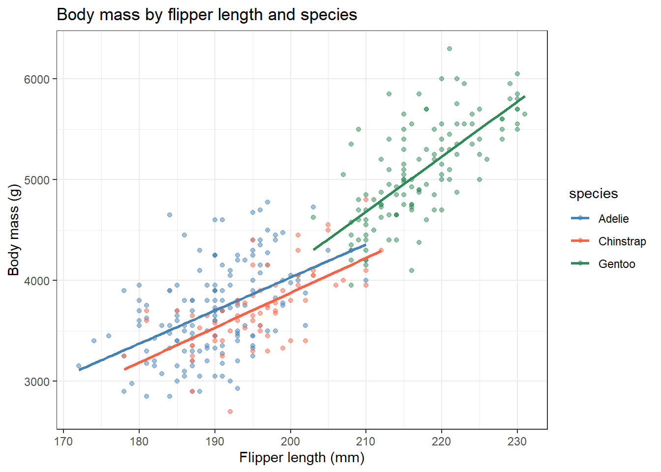

NoteWhere to Find Data Like This

PBC dataset: survival::pbc: multiple correlated clinical predictors with a continuous outcome, ideal for demonstrating confounding and model building.

palmerpenguins: palmerpenguins::penguins: biological measurements with species as a natural confounder.

NHANES: Many continuous health outcomes (blood pressure, cholesterol) with multiple demographic and clinical predictors.

12.7 What Can Go Wrong

Estimated time: ~10 minutes (reading)

Warning

Overfitting. Adding more predictors always increases R². Use adjusted R², AIC, or cross-validation to compare models, not raw R².

Multicollinearity. Highly correlated predictors produce inflated standard errors and unstable coefficients. Check VIF before interpreting a model with many predictors.

Including colliders. Adjusting for a variable on the causal pathway between exposure and outcome (a mediator) or a common effect of both (a collider) can introduce bias. See the Causal Inference session for guidance.

Data-dredging. Selecting predictors based on p-values from exploratory analysis, then reporting the final model as if it were pre-specified, produces overfitted models with inflated associations. Pre-register your model or use a penalised method (ridge, lasso).

Interpreting coefficients in models with interactions. When an interaction is present, the main effect coefficients are conditional on the other variable being at its reference level, not the marginal effect. Always evaluate interactions at meaningful covariate values.

WarningCommon Misinterpretations

“Adding more predictors always improves my model.” Raw R² always increases with more predictors, even if they are noise. Use adjusted R², AIC, or cross-validation. A model with 20 predictors and 50 patients is almost certainly overfitted.

“My predictor is not significant so it has no effect.” With collinear predictors, both can become non-significant even if together they explain a lot of variance. Check VIF and consider whether the predictors should be modelled together or separately.

“The adjusted model is always more accurate than the unadjusted one.” Adjusting for a collider introduces bias that was not there in the unadjusted model. Think carefully about the causal structure before adding covariates. See the Causal Inference session.

“I can compare R² between models with different outcomes.” R² is not comparable across different outcome variables or different datasets. Only compare R² (or AIC) between models fitted to the same data with the same outcome.

“Stage 2 coefficient = −0.11 means Stage 2 patients have lower albumin.” It means Stage 2 patients have 0.11 g/dL lower albumin than Stage 1 patients after adjusting for other predictors – and in our fit_full model, this particular difference was not statistically significant (p ≈ 0.24). Change the reference category and the coefficient changes. Always state the reference group when reporting factor coefficients.

NoteTeacher Note

A quick true/false check before moving to the exercises:

1. “If a predictor’s coefficient is not significant in the full model, it has no effect on the outcome.” False – with correlated predictors, an effect can be shared across several variables so that none individually reaches significance, even though jointly they matter (see the LRT for stage, p < 0.001).
2. “Adding more predictors will always increase R².” True for raw R² – but adjusted R², AIC, and BIC penalise added complexity, which is why we compare models on those instead.
3. “A coefficient that shrinks after adjustment was previously biased by confounding.” Often true, but not certain – shrinkage is consistent with confounding, but could also reflect chance variation or a collider; the causal interpretation depends on subject-matter knowledge, not the regression output alone.

12.8 Exercises

NoteTeacher Note

Pair learners up for Exercise 1 and 2. For Exercise 1, ask them to predict the order of the three models by AIC before running the code – most will correctly guess that the full model (with stage) has the lowest AIC, echoing the LRT result from Example 1. For Exercise 2, ask whether they expect the flipper-length-by-species interaction to be significant; the answer (yes, driven mainly by Gentoo) reinforces that “adjusting for species” (Example 2) and “letting the slope vary by species” (this exercise) are related but different questions.

12.8.1 Exercise 1 (Guided): Build and Compare Models

Estimated time: ~15 minutes

Using pbc, predict albumin from:

1. Univariable: log_bili only
2. Multivariable: log_bili + log_proto
3. Full: log_bili + log_proto + stage

Report adjusted R² and AIC for each model. Which is best? Does adding stage improve fit (use anova())?

TipExercise 1: Solution

m1 <- lm(albumin ~ log_bili, data = pbc)
m2 <- lm(albumin ~ log_bili + log_proto, data = pbc)
m3 <- lm(albumin ~ log_bili + log_proto + stage, data = pbc)

bind_rows(
  glance(m1) %>% mutate(model = "1: log_bili"),
  glance(m2) %>% mutate(model = "2: + log_proto"),
  glance(m3) %>% mutate(model = "3: + stage")
) %>%
  select(model, adj.r.squared, AIC)

# A tibble: 3 × 3
  model          adj.r.squared   AIC
  <chr>                  <dbl> <dbl>
1 1: log_bili            0.122  408.
2 2: + log_proto         0.132  404.
3 3: + stage             0.183  382.

anova(m2, m3)

Analysis of Variance Table

Model 1: albumin ~ log_bili + log_proto
Model 2: albumin ~ log_bili + log_proto + stage
  Res.Df    RSS Df Sum of Sq     F    Pr(>F)    
1    407 63.012                                 
2    404 58.878  3    4.1343 9.456 4.738e-06 ***
---
Signif. codes:  0 '***' 0.001 '**' 0.01 '*' 0.05 '.' 0.1 ' ' 1

Run the chunk above. Adjusted R² rises from about 0.122 (model 1) to 0.132 (model 2) to 0.183 (model 3), while AIC drops from about 408 to 404 to 382. By both criteria, model 3 (with stage) is best. anova(m2, m3) gives F = 9.456, p = 4.738e-06: adding stage significantly improves the fit beyond log_bili + log_proto alone.

12.8.2 Exercise 2 (Semi-guided): Penguin Model with Interaction

Estimated time: ~15 minutes

Using palmerpenguins::penguins, fit a model predicting body mass from flipper length, species, and their interaction.

1. Fit lm(body_mass_g ~ flipper_length_mm * species, data = penguins).
2. Is the interaction significant? Check using anova().
3. Interpret: does the slope of flipper length differ between species?

TipExercise 2: Solution

peng3  <- penguins %>% drop_na()
fit_i  <- lm(body_mass_g ~ flipper_length_mm * species, data = peng3)
fit_no <- lm(body_mass_g ~ flipper_length_mm + species,  data = peng3)

anova(fit_no, fit_i)

Analysis of Variance Table

Model 1: body_mass_g ~ flipper_length_mm + species
Model 2: body_mass_g ~ flipper_length_mm * species
  Res.Df      RSS Df Sum of Sq     F   Pr(>F)   
1    329 45843144                               
2    327 44391669  2   1451475 5.346 0.005193 **
---
Signif. codes:  0 '***' 0.001 '**' 0.01 '*' 0.05 '.' 0.1 ' ' 1

tidy(fit_i, conf.int = TRUE) %>%
  filter(str_detect(term, "flipper")) %>%
  select(term, estimate, conf.low, conf.high, p.value)

# A tibble: 3 × 5
  term                               estimate conf.low conf.high  p.value
  <chr>                                 <dbl>    <dbl>     <dbl>    <dbl>
1 flipper_length_mm                     32.7     23.5       41.9 1.78e-11
2 flipper_length_mm:speciesChinstrap     1.88   -13.6       17.4 8.11e- 1
3 flipper_length_mm:speciesGentoo       21.5      7.77      35.2 2.23e- 3

Run the chunk above. anova(fit_no, fit_i) gives F = 5.346, p = 0.0052: the interaction is statistically significant overall. Looking at the coefficients, the flipper-length slope for Adelie (the reference species) is about 32.7 g/mm. The interaction term for Chinstrap is small and not significant (≈ 1.9, p = 0.81), but for Gentoo it is about 21.5 (95% CI: 7.8 to 35.2, p = 0.002) – meaning Gentoo’s flipper-mass slope (≈ 32.7 + 21.5 ≈ 54.2 g/mm) is significantly steeper than Adelie’s or Chinstrap’s. The interaction is “significant” mainly because Gentoo behaves differently, not because all three species differ from each other.

12.8.3 Exercise 3 (Open-ended)

Estimated time: 15–30 minutes

In your own research, identify a continuous outcome with at least two potential predictors. Fit univariable and multivariable models. Compare the coefficients: do they change after adjustment? Interpret any changes as confounding and write a Methods section justifying your final model.

12.9 Comprehension Check

Estimated time: ~10 minutes (self-test)

1. You fit a simple regression and get slope = −0.5 for log_bili. In the multivariable model with protime and stage, the slope is −0.2. What happened, and what does this tell you?
2. VIF for two of your predictors is 12 and 11. What is the problem, and what are your options?
3. You compare two models with anova() and get p = 0.0003. What does this mean?
4. A colleague says “AIC is lower for Model B, so Model B is definitely correct.” Is this right?
5. An interaction term has estimate = 0.15, 95% CI (−0.02, 0.32), p = 0.08. Should you include it in the final model?

NoteAnswers

1. The simple regression slope was confounded: bilirubin was acting partly as a proxy for prothrombin time and disease stage. After adjustment, the partial effect of bilirubin is smaller (−0.2), reflecting the unique contribution of bilirubin above and beyond the other predictors.
2. VIF > 10 indicates severe multicollinearity. The two predictors are so highly correlated that their individual coefficients are unreliable (large SEs, may flip sign). Options: (1) remove one of the correlated predictors; (2) combine them into a composite score; (3) use ridge regression, which handles multicollinearity by regularisation.
3. The F-test comparing the two models is highly significant; the larger model fits significantly better than the smaller model. At least one of the additional predictors contributes meaningfully.
4. No. AIC is a relative measure of model quality penalised for complexity. Lower AIC means a better fit-to-complexity balance among the models compared, but it does not guarantee the model is “correct” in an absolute sense.
5. The evidence is weak and the CI includes zero. Whether to include it depends on context: if it was pre-specified with a plausible biological rationale, you might retain it and acknowledge the marginal evidence. If it was data-driven, it is safer to use the main-effects model.

12.10 How to Report

Note

In a methods section: “A multiple linear regression model was built with [outcome] as the dependent variable. Candidate predictors included [list]. Variables were selected based on [method: biological rationale / stepwise / LASSO]. Variance inflation factors (VIF) were examined to assess multicollinearity.”

In results: “After adjustment for [covariates], [predictor] remained independently associated with [outcome] (β = X, 95% CI [L, U], p = Y). The full model explained X% of the variance in [outcome] (adjusted R² = X).”

Always include:

• Coefficients (β) with 95% CI for each predictor
• Overall model fit (adjusted R²)
• n and number of predictors (flag if n/predictor ratio < 10)
• Variable selection method used

Never report unadjusted and adjusted estimates in the same sentence without clearly labelling which is which.

12.11 Further Reading

• Dalgaard (2008): Multiple regression chapter in Introductory Statistics with R
• Bland (2015): Multivariable regression in An Introduction to Medical Statistics
• ?lm, ?vif (from car), ?anova.lm in R
• Harrell (2015): Regression Modeling Strategies, a comprehensive reference for clinical regression

Bland, Martin. 2015. An Introduction to Medical Statistics. 4th ed. Oxford University Press.

Dalgaard, Peter. 2008. Introductory Statistics with r. 2nd ed. Springer.

Harrell, Frank E. 2015. Regression Modeling Strategies. 2nd ed. Springer.